Useful Equations Glossary

---

Table of Contents

• Multivariable Calculus
• Differential Equations
• Complex Analysis
• Graph Theory
• Matrix Methods
• Fourier Analysis
• Mechanics
• Electrostatics
• Diffusion
• Electrochemistry
• Quantum Chemistry
• Computational Neuroscience
• Probability
• Information Theory
• Electrical Engineering

---

Multivariable Calculus

Line integrals in a scalar field give the area under a space curve. The formula can be generalized for more variables.

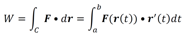
When a line integral is taken using a vector field, the work performed by the vector field on a particle moving along a space curve in the field can be computed. This is applicable to numerous analogous situations as well. The line integral in a vector field is given by the equation below. F defines the vector field and the curve C is a vector function given by r(t).

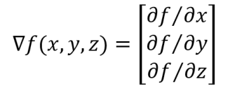
The gradient is the vector of the partial derivatives of a function with respect to each of its variables.

The gradient can be operated on in a variety of ways. For instance, the dot product of the gradient and a unit vector gives the directional derivative (the rate of change in the direction of that unit vector).

Divergence is a measure of the “flow” emerging from any point in a vector field. Positive divergence indicates a “source,” while negative divergence indicates a “sink.”

Curl describes the amount of counterclockwise rotation around any point in a vector field. Positive curl indicates more counterclockwise rotation, while negative curl indicates more clockwise rotation. 2D curl has a simple formula (below, top) and 3D curl has a somewhat more complicated formula (below, bottom).

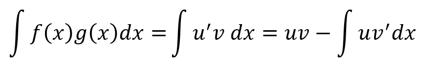
Integration by parts is a way to “reverse the product rule.” For integration by parts, let f(x)=u‘ and g(x)=v.

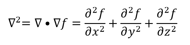
The Laplacian is the sum of unmixed second partial derivatives of a multivariable function. Roughly speaking evaluating the Laplacian at a point measures the “degree to which that point acts as a minimum.” Consider f(x,y,z). When a high positive value comes from evaluating the Laplacian at a point, that point will likely have a lower value for f than most of the neighboring points.    

Differential Equations

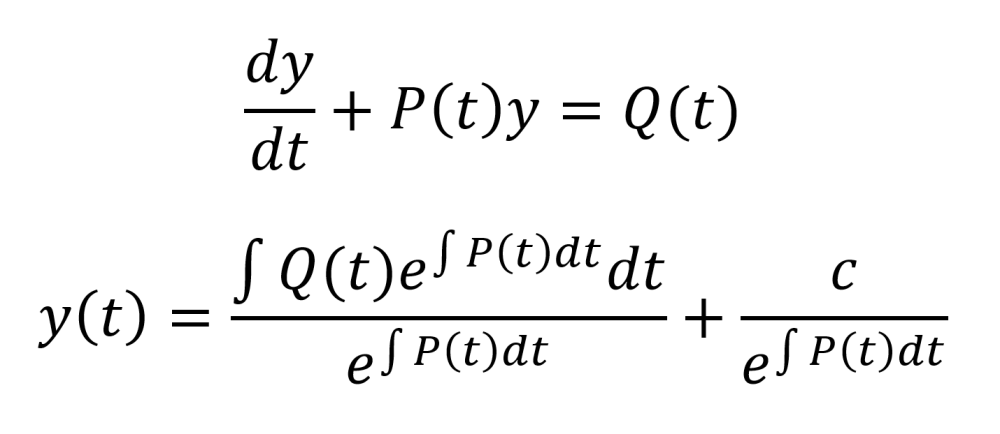
Given a first order linear differential equation that can be arranged into the form given by the top equation below, the solution to that differential equation is given by the bottom equation below.

The Laplace transform is useful for solving differential equations with known initial values for y(t), y’(t), y’’(t), and any higher order derivatives present. It is defined by the top equation, but it is often easier to employ tables of Laplace transforms of common functions and modify the results for the problem of interest. Laplace transforms have a variety of useful properties described by the rest of the equations below. Furthermore, the Laplace transform is a linear operator.

Complex Analysis

Euler’s identity relates e, i, and ϴ to trigonometric functions.

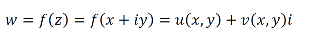
For a complex valued function, f(z) = w, the complex variable z maps to another complex variable w. Complex valued functions can be described as a transformation from a point (x,y) to a point (u,v) as given by the equation below.

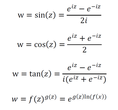
Trigonometric functions of a complex variable z can be represented in terms of exponentials. In addition, a complex function f(z) raised to the power of another complex function g(z) may be expressed as the bottom equation.

Complex integrals are also called contour integrals. Integrals of complex functions can be expressed in terms of line integrals if f(z) is continuous on a parameterized space curve.

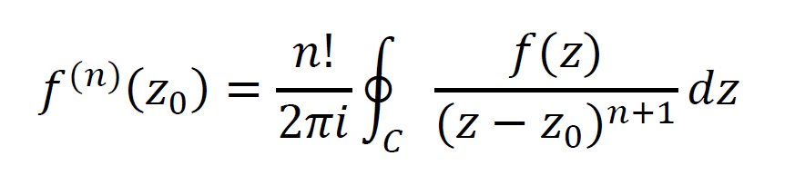
Cauchy’s integral formula states that, for a simply connected domain D and a curve C which lies within D and contains a point z₀, the equation below holds. (Simply connected domains have no “holes” and their boundaries do not cross each other).

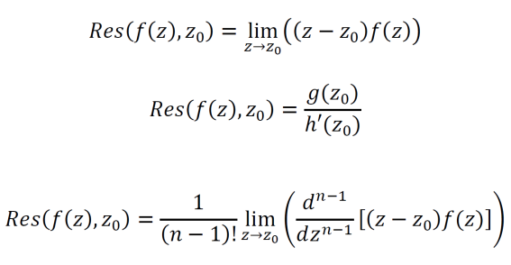
In complex analysis, residues come from a generalized (to complex numbers) version of Taylor series called Laurent series. They are useful in evaluating contour integrals. If the complex part of a Laurent series contains a finite number of terms, then z = z₀ is called a pole of order n. Here, n is the power to which (z – z₀) is raised in the denominator of that term in the given Laurent series. If n=1, the pole is called a simple pole and can be computed by the formulas at top or middle. For higher order poles, the formula at bottom can compute the residue.

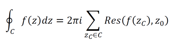
Cauchy’s residue theorem requires a simply connected domain D with a closed contour C inside and a function f(z) which is differentiable on and within C except at a finite number of points z₁, z₂, … z_n. If these conditions are met then, the contour integral of f(z) may be computed by the equation below.

 

Graph Theory

The handshaking lemma states that, for any graph G(V,E), the sum of the node degrees equals twice the number of edges.

Euler’s formula holds for simple (undirected and no self-edges) planar graphs. Planar graphs are graphs that can be represented without any edges crossing each other. V represents the number of nodes, E represents the number of edges, and F represents the number of faces including the infinite face outside of the graph.Euler’s formula holds for simple (undirected and no self-edges) planar graphs. Planar graphs are graphs that can be represented without any edges crossing each other. V represents the number of nodes, E represents the number of edges, and F represents the number of faces including the infinite face outside of the graph.

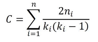
The clustering coefficient for a graph is given below. Here, n is the number of edges among the neighbors of node i and k is the number of neighbors of node i.

 

Matrix Methods

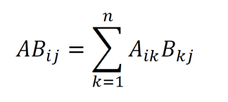
The matrix product is described by the equation below. Note that the inner dimensions of the matrices must match for the matrix product to be defined.

The transpose of any matrix is applied as in the example below.

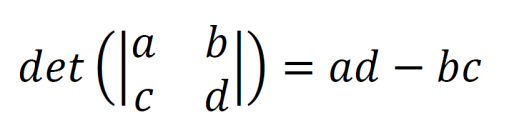
The determinant of a 2×2 matrix is given by the equation below.

Eigenvalues and eigenvectors are very useful for a variety of applications. They are related to a matrix A and a vector x by the equation at top. To find the eigenvalues of a matrix, apply the formula at middle and find the zeros of the resulting polynomial. The zeros are the eigenvalues of the matrix. The eigenvectors of an eigenvalue can be found by solving the system at bottom for x₁…x_n. The set of all scalar multiples of the solved vector [x₁…x_n] is the set of eigenvectors for the given eigenvalue.

 

Fourier Analysis

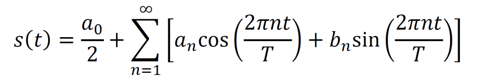
Fourier series are weighted sums of sines and cosines that can represent any periodic signal. Here, the period of signal s is given by T.

The Fourier series coefficients are the weights of the sines and cosines. They are given by the integrals below.

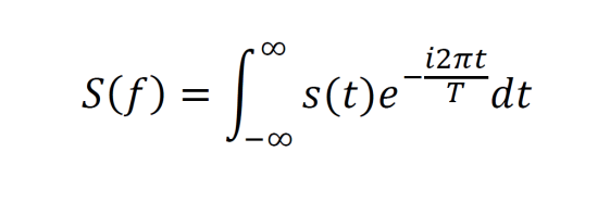
The continuous Fourier transform takes in a signal function s(t) and decomposes it into its component weighted sines and cosines. It employs the relationship between complex numbers, sines, and cosines to achieve this. Fourier transforms are said to convert from the time domain to the frequency domain. By observing the frequency domain, a signal can be more easily analyzed and decoded.

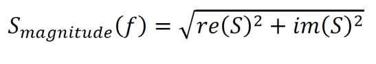
Since the output of a Fourier transform is usually complex, the equation below can be used to convert the output to a power spectrum.

The signal can be reconstructed using the inverse Fourier transform. This is useful in data compression since the data can undergo a Fourier transform and then later be reconstructed using the inverse Fourier transform, given below.

The discrete Fourier transform has the same purpose as the continuous version, but it operates on discrete data s(k) and so uses summation rather than integration.

Power spectra can also be computed for discrete Fourier transforms.

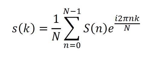
By applying the discrete Fourier transform and then the inverse discrete Fourier transform (below), a discrete signal can be compressed and then reconstructed.

 

Mechanics

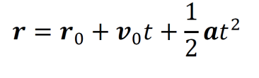
Multidimensional equation of motion (constant acceleration).

Momentum in kg•ms^-1 (top), work in J given constant force (middle), circular motion at constant speed (bottom).

Newton’s second law in terms of mass and acceleration (top) and in terms of momentum (bottom). Force is measured in Newtons.

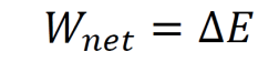
Work-energy theorem.

Velocity of an object undergoing circular motion given its period.

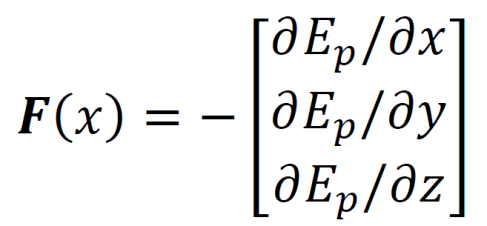
Force from potential energy in 3D.

Potential energy function for spring (top) and spring force formula (bottom).

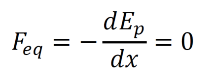
Objects move to minimize their potential energy. When the net force is zero, so is the derivative of the potential energy. Note that stable and unstable fixed points apply here.

Energy of isolated system with thermal energy U.

Multidimensional power with constant force. Power is measured in J/s.

Multidimensional work with variable force (given by a vector field) as a line integral.

 

Electrostatics

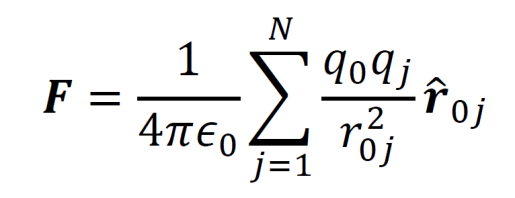
Suppose that a constellation of point charges exists at a given time. If a new charge, q₀ is brought into the vicinity of the other charges and placed at a location x,y,z, then the force from the other charges on q₀ is given by the equation below. The ȓ_0j represents a unit vector extending from q_j to the point x,y,z. The ϵ₀ represents a constant known as the permittivity of free space and is equal to 8.85•10^-12.

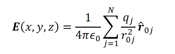
The electric field in the above scenario is defined as the equation below, where F has been divided by q₀.

To calculate the electric field from a continuous charge distribution at a point x₀,y₀,z₀, the triple integral below is used over the volume region D. The unit vector ȓ points from (x,y,z) to (x₀,y₀,z₀).

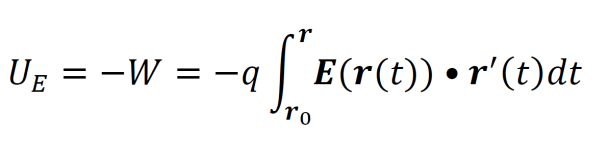
The electrostatic potential energy of a point charge q brought into the vicinity of an electric field E is given by a line integral describing the work performed on the point charge to move it from position r₀ to r.

Given an electrostatic potential function U_E, the electric field is given by the gradient of U_E.

 

Diffusion

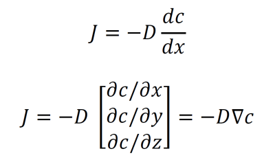
Fick’s first law of diffusion describes the relationship between the flux J of particles across an area and the concentration of the particles. D is a proportionality constant called the diffusion coefficient. The law is given in 1D at top and in 3D at bottom.

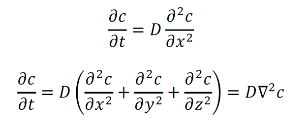
Fick’s second law of diffusion describes how particles flow given a concentration gradient. The law is given in 1D at top and in 3D at bottom. This is equivalent to the heat equation.

 

Electrochemistry

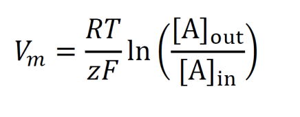
The Nernst equation describes the membrane voltage given an ion’s concentration on each side of the membrane. R is the gas constant (8.314 J/K), F is Faraday’s constant (96,485 C/mol), z is the charge of the ion, and T is the temperature in Kelvin.

The Goldman equation expresses the membrane voltage given multiple types of ions and relative permeabilities of the membrane to those ions.

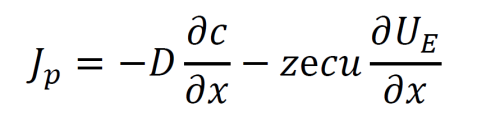
The Nernst-Planck equation describes ion flow with electrical potential and concentration gradients. J_p indicates particle flux over an area, D is a diffusion coefficient, U_E is the electrical potential, e represents the elementary charge of 1.6•10^-19 C, z is the charge of the given type of ion, and u is the mobility constant of the ion in the solution.

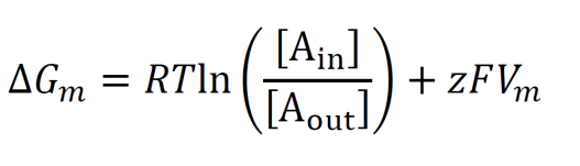
The free energy required for an ion to cross a semipermeable membrane (like a phospholipid membrane) is given by the equation below. This equation accounts for a preexisting membrane voltage from another ion. If the free energy is negative, the ions in the first term will spontaneously cross the semipermeable membrane. Note that the numerator and denominator within the natural logarithm are switched relative to the Nernst equation.

 

Quantum Chemistry

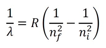
The Rydberg equation gives the wavelength emitted when an electron moves from an excited state n_i to a lower energy level n_f. Here, R is the Rydberg constant, 1.097•10⁷ m^-1.

Given an electromagnetic wave, its velocity (the speed of light c), frequency, and wavelength are related by the equation below.

Particles have wavelengths known as de Broglie wavelengths. They can be computed using Planck’s constant 6.626•10^-34 m²kg/s over the momentum mv.

The energy of a wave (in J) is given by the formulas below. Note that frequency is equivalent to c/λ.

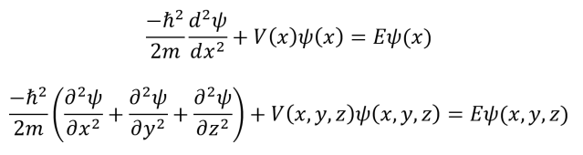
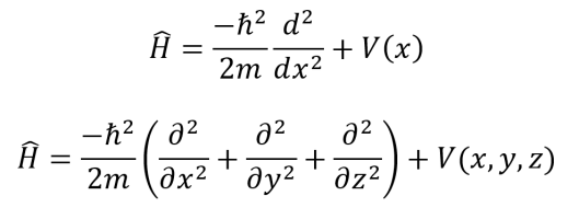
The time independent Schrödinger equation relates the wavefunctions of a particle and its energy. Solving this equation gives a formula for the wavefunction of a given particle. The symbol  represents h/2π. V(x) is the potential energy, m is the mass, and E is the energy. The 1D version is shown at top and the 3D version is shown at bottom.

The Hamiltonian operator describes the kinetic and potential energy of a quantum system. It can be applied to wavefunctions to generate the Schrödinger equation. The Hamiltonian in 1D is given at top and the Hamiltonian in 3D is given at bottom.

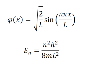
The wavefunction solution of a 1D particle in a box with boundary conditions ψ(0)=0 and ψ(L)=0 is given at top. The n represents the discrete energy level of the particle and may take on values of 1,2,3… The energy of the particle at energy level n is given at bottom.

The wavefunction solution of a 3D particle in a box with boundary conditions ψ(0,y,z)=0, ψ(L_x,y,z)=0, ψ(x,0,z)=0, ψ(x,L_y,z)=0, ψ(x,y,0)=0, ψ(x,y,L_z)=0 is given at top. The n_x, n_y, and n_z represent the x,y,z components of the particle’s discrete energy level n. Each component must still be a poösitive integer. The energy of the particle at energy level n is given at bottom.

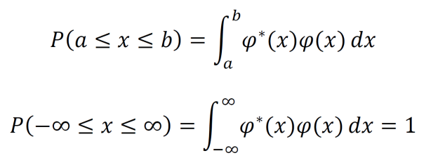
The integral of the wavefunction squared denotes the probability that a particle will be found within a given region. Since wavefunctions may be complex, the square must be computed using the complex conjugate. This is the 1D version of the equation.

The average or expectation value of a measurable property (associated with an operator) is given in 1D and 3D by the integrals below. Note that the integral in the denominator acts to normalize the result.

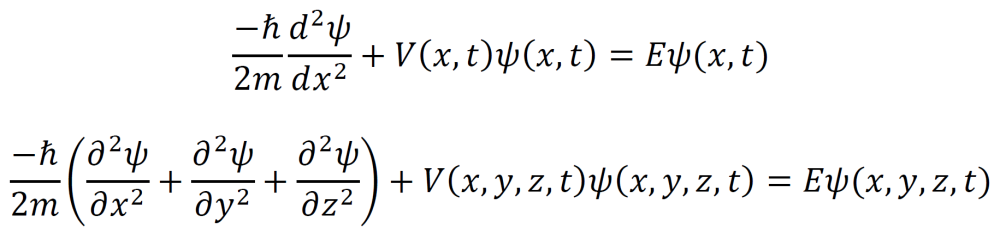
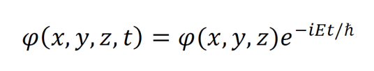
The time-dependent Schrödinger equation describes the evolution of a wavefunction over time.

The general solution to the time-dependent Schrödinger equation is the time-independent wavefunction times a complex exponential.

 

Computational Neuroscience

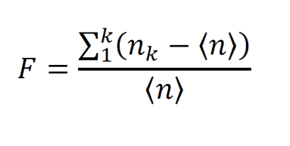
Consider the spikes of a single neuron being recorded over a time interval t. This experiment is carried out for K trials. The firing rate v in trial k is given by the number of spikes over t. Repeating the experiment several times allows the repeatability of the spike count n_k across repetitions to be calculated. This variability, the Fano Factor, is the variance of the spike count over the mean spike count.

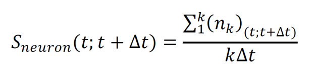
To construct a peri-stimulus-time histogram, consider a spike train over time interval t with k trials. Split the interval into subintervals (t; t + ∆t) and sum the number of spikes over all trials within each subinterval. Then divide by k∆t, the number of trials times the size of each subinterval. 

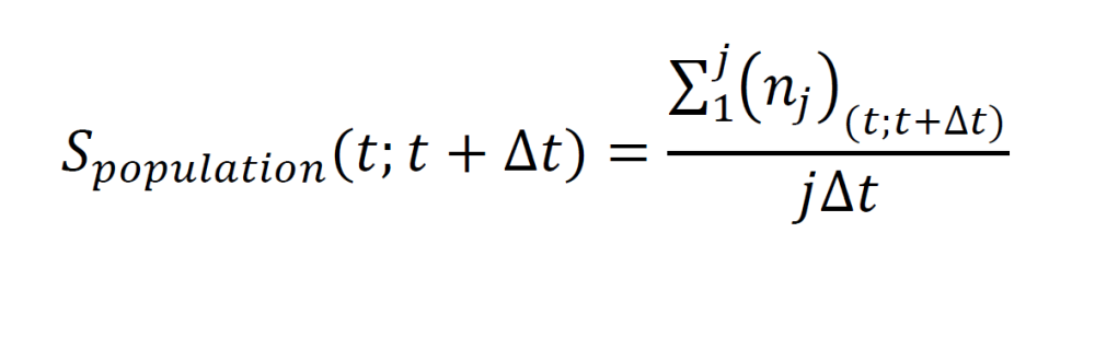
Average neural population activity can be computed from simultaneously measuring of j different neurons over a time interval t. Split the time interval into subintervals (t; t + ∆t) and sum the number of spikes over the whole population for each subinterval. Then divide by j∆t to obtain the average population activities at each subinterval.

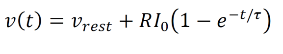
Integrate-and-fire neurons are modeled by a linear differential equation. The solution to that differential equation given an initial condition v(0) = v_rest is shown below. The variable v represents the membrane voltage, R is the membrane resistance, I₀ is the injected current, and τ is a time constant for the membrane. When using integrate-and-fire neurons, a firing threshold is often set.

The Hodgkin-Huxley equations are a system of differential equations that model neural electrophysiology. The system must be solved numerically. The C(dv/dt) term, in which capacitance is multiplied by the change in voltage with respect to time, is equivalent to current across the membrane. Note that membrane voltage is a function of time. E_ion is the equilibrium potential for that ion across the membrane, I_in is the injected current, and g_ion is the conductance value for that ion across the membrane. The parameters m, n, and h help describe the gating of the ion channels and fit the model to data.

 

Probability

Conditional probability (the probability of B happening given A).

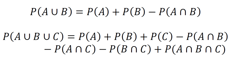
Joint probability (the probability of A and B occurring). This is described using an intersection. Joint probability for three events and four events is also given. Further extrapolation follows the same pattern.

The probability of A or B, but not both (described using a union). The probability of A, B, or C but not any other combination of the events is also given. Further extrapolation follows the same pattern.

Bayes theorem gives the probability of an event based on prior knowledge of other conditions that may have influence on the event.

For a discrete random variable, a probability mass function gives the probability associated with each outcome of a random experiment.

Cumulative distribution functions (CDFs) give the probability that a random variable X will give a value less than or equal to x.

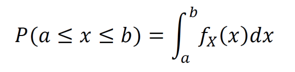
For a continuous random variable, the integral of a probability density function f_X gives the probability that the outcome lies on the chosen interval.

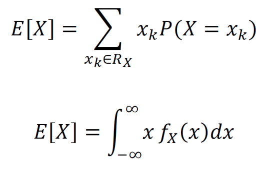
The expected value is the average of each outcome times its probability. The discrete case is given at top and the continuous case is given at bottom.

The variance is a measure of the spread of data. The square root of variance is standard deviation. The general equation for variance is given at top. To compute discrete variance, use the equation at middle. To compute continuous variance, use the equation at bottom.

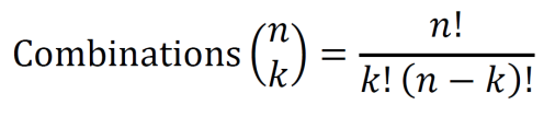
Given a set of n total elements, a permutation is a selection of k elements from the set such that the order does matter. The number of permutations of a set is given below.

Given a set of n total elements, a combination is a selection of k elements from the set such that the order does not matter. The number of combinations of a set is given below.

 

Information Theory

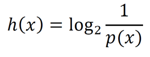
Shannon information is a measure of “surprise” associated with an outcome. The units are bits and p(x) is the probability of the given outcome.

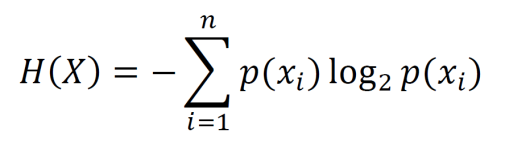
Entropy is the average amount of Shannon information from a stochastic data source.

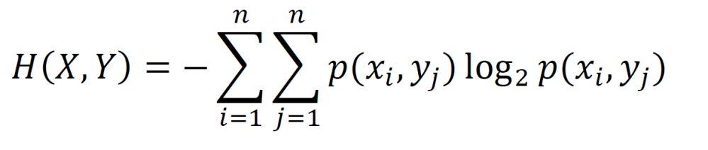
Joint entropy is the entropy for multiple random variables (the joint entropy for two random variables is given below).

Conditional entropy is the entropy of X given that a particular outcome y (from the other variable) is known.

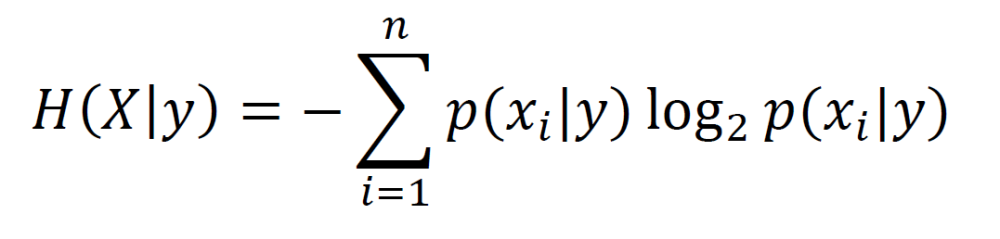
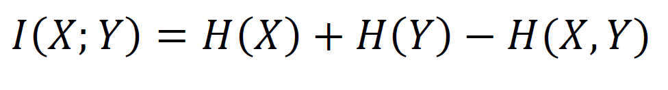
Mutual information measures the mutual dependence of two random variables. It does not necessarily imply causality, though sometimes it is associated with causality. The mutual information I(X;Y) is given by the sum of individual entropies minus the joint entropy.

 

Electrical Engineering

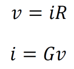
Electrical current is defined as the amount of charge in Coulombs that flows through a conductor or circuit element per unit time. The Coulomb is a unit of charge that is equivalent to 1.602•10¹⁹ elementary charges. One electron has a charge of -1.602•10^-19 C. Current is measured in amperes, which are C/s. Voltage is defined as the amount of energy per unit charge that moves through a given circuit element. It is measured in J/C or volts. Voltage can be thought of as electrical potential energy. Resistance has units of V/A or ohms, represented by Ω. Current, voltage, and resistance are related by Ohm’s law (top). Conductance refers to the inverse of resistance, is represented by G, and is measured in inverse ohms Ω^-1 or siemens S. Ohm’s law in terms of conductance is given at bottom.

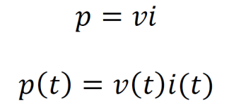
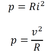
Power is the rate of energy transfer in J/s or watts. Power is given by the product of current and voltage.

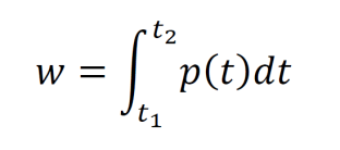
Energy delivered to a circuit element is computed by integrating power over a time interval.

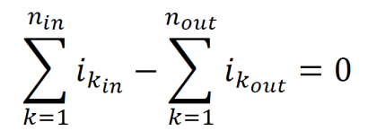
Kirchhoff’s current law states that the net current entering a node equals zero. The net current equals the sum of currents entering minus the sum of currents leaving. Alternatively, this law states that the sum of the currents entering a node equals the sum of the currents leaving the node. If several circuit elements are connected to a pair of nodes which are themselves connected, then the circuit elements can be considered as connected to a common node.

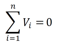
The closed path from a node, through some circuit elements, and back to the same node is called a loop. Kirchhoff’s voltage law states that the sum of the voltage changes around a closed loop in a circuit equals zero. If the path taken around the loop starts in the direction of a circuit element that undergoes a voltage drop, that circuit element is given a positive value. If the path starts by crossing a circuit element such that there is a voltage gain, that circuit element is given a negative value.

If the length L of a resistor is much larger than its cross sectional area A, then the resistance can be approximated by the formula below. The letter ρ is a constant for the material of the given resistor called the resistivity. The resistivity is measured in ohm meters Ωm.

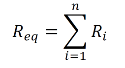
Resistances in series can be summed into a single resistance. This single equivalent resistance can replace the original set of resistances in the analysis.

Resistances in parallel can be converted into a single equivalent resistance using the equation below.

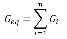
The equation for conductance in series is given below.

The equation for conductance in parallel is given below.

The capacitance for a parallel plate capacitor, measured in Farads (coulombs per volt), is given by the equation below. Here, ε is the dielectric constant for the material between the plates, A is measured in square meters, and d is measured in meters.