The Promise of Psychiatric Gene Therapy
Current psychiatric interventions remain insufficient to address the highly prevalent mental illnesses which plague more than a billion people (1 in 7) across the world.1 Widespread and debilitating diseases like major depressive disorder (MDD),2 anxiety disorders,3 schizophrenia,4 bipolar disorders,5 post-traumatic stress disorder (PTSD),6 substance abuse disorders,7,8 and personality disorders9,10 pose an enormous global health burden and are one of the most central causes of human suffering. Patients frequently do not respond to pharmacological interventions for these conditions, resulting in vast numbers of people struggling through life without options for proper management. As a result, at least 800K people die by suicide annually.11 Today’s neuropharmacology industry employs small molecule drugs which modulate neurochemical states, utilizing strategies like neurotransmitter reuptake inhibition and receptor agonism. Mechanistic underpinnings of many neuropharmacological treatments are not well understood.2,12 Furthermore, small molecules suffer from extensive off-target binding13 and frequently come with side effects, many of which can be extremely debilitating and/or dangerous. Though it has been cemented into place by partial successes,12 the way we currently treat mental illnesses is woefully inadequate.
Why might gene therapy solutions eventually offer better treatment options for common psychiatric disorders compared to traditional small molecule pharmaceuticals? Gene therapies possess a number of intrinsic advantages like cell-type-specific targetability, direct in situ expression of therapeutic proteins or RNAs, and the capacity to dynamically respond to environmental conditions. They also have potential for spatiotemporal programmability via emerging sonogenetics14–17 and chemogenetics18 approaches. (Sonogenetics has particular promise, which will be discussed in more detail later). In addition, gene therapies may be engineered to downregulate (RNAi or CRISPRi)19 or even ablate (CRISPR knockout)20 expression of almost any gene in the genome, offering an unprecedented array of new therapeutic targets. CRISPRa might also be employed to upregulate target genes without altering the genome.19 Engineering gene therapies which express multiple proteins or RNAs at once may synergistically improve efficacy.21,22 Importantly, gene therapies can be engineered to persist for long periods of time23,24 or to only provide a burst of short term expression. Depending on the genetic payload, one or the other of these durations may represent the most optimal choice. Gene therapies altogether provide a much larger space of possibilities for precision alteration of brain states than has been possible for small molecule treatments. I would argue that this space’s capabilities remain severely underexplored primarily because of a lack of delivery system capabilities.
Better Delivery Systems are Needed
Gene therapy promises to open a new world of precision psychiatric treatments, yet its potential has gone unrealized. This makes sense as there are a number of obstacles which render psychiatric gene therapy a difficult target. Among these, the challenges of brain delivery, safety, and manufacturing scalability represent particularly recalcitrant bottlenecks. Adeno-associated virus (AAV) gene therapies have progressed furthest in the brain delivery field. Industry players like 4DMT, Dyno Therapeutics, Apertura Therapeutics, and Capsida Biotherapeutics have made efforts via directed evolution, rational design, and machine learning towards optimizing AAV capsids for blood-brain-barrier (BBB) crossing efficiency. However, safety concerns stemming from several patient deaths in systemically administered AAV therapies over the past few years have slowed this progress. Additionally, limitations in AAV manufacturing capacity pose a problem for scaling the vector to populations of 1M+ patients.25 This will be discussed in more detail further on. It should be noted as well that AAVs are limited by their small DNA packaging capacity of 4.7 kb. To unlock the potential of psychiatric gene therapy, we need safer and more scalable delivery systems.
Although there exist multiple obstacles to overcome before gene therapy can realize its potential as a psychiatric modality, I propose a lack of delivery systems represents a foundational missing piece. Without strong delivery vehicles to feasibilize solutions, the field of psychiatric gene therapy will not be credible enough to receive substantial investment. It is a “tools problem”. As mentioned earlier, there is a particular need for vectors which at once possess high safety, scalability, and efficacy. I strongly suspect that the emergence of vectors with these qualities would seed an explosion of efforts towards gene therapies for brain diseases, which would eventually allow us to tackle psychiatric ailments. While psychiatric diseases are unlikely to represent the initial targets of brain gene therapies, opening the door to brain delivery will in my view be necessary to take steps in the direction of modernizing psychiatry through precision genetic medicines.
Examination of the Current Landscape
As mentioned earlier, AAV gene therapies are the current frontrunner for brain delivery yet possess both scalability and safety limitations. I will explain the scalability issue using publicly available information on AAV manufacturing: Final yields (after purification) of AAVs have been reported or modeled in scientific literature with values ranging from around 7.5×10¹² vg/L to 7.5×10¹³ vg/L.26–28 I will thus assume here that 5×10¹³ vg/L is a typical yield. For this rough calculation, I will also assume that the yield scales linearly with bioreactor volume. As such, a 2,000 L bioreactor would make batches of around 1017 vg and a 200 L bioreactor would make batches of around 1016 vg. According to a 2024 report, a 200 L AAV production run at cGMP quality costs about $2M (including analytics).29A 2022 meta-analysis study of clinical AAV doses states that per patient systemic delivery amounts range from 3.5×10¹³ vg total to 1.5×10¹⁷ vg total.30 Huang et al.’s highly promising AAV BIhTFR1 capsid (the basis for Apertura Therapeutics) was originally administered to mice at a higher dose of 1014 vg/kg and a lower dose of 5×10¹² vg/kg.31 Generously (perhaps too generously) assuming that the lower dose is sufficient, this would equate to about 4×10¹⁴ vg total in an average 80.7 kg North American adult human.32 Dividing 1016 vg from a $2M (200 L) batch by 4×10¹⁴ vg per dose, this means each batch would provide 25 doses for about $80,000 each. Even if substantial improvements in manufacturing yield and in lowering required dosage happen, I am skeptical that systemic AAV approaches will scale to disease indications with 1M+ patients. Despite this, AAVs remain still a central point in the gene therapy industry for a reason and paradigm-shifting approaches to manufacturing25 and/or efficacy might still change the current scalability challenges.
Another existing modality is transient focused ultrasound BBB opening (BBBO). I would argue that BBBO is extremely promising for some applications but not a universal solution. Treatment of many brain diseases necessitates brain-wide delivery. By contrast, BBBO is generally a localized delivery technique.33 Although some common psychiatric diseases fit these parameters, most common ailments with clean clinical endpoints do not. Some work has been done to extend BBBO ultrasound to larger-volume delivery through multiple sonication34,35 or raster scanning,36 but this remains much less well-developed by comparison to localized BBBO approaches and may exhibit greater safety concerns. Indeed, while single-site BBBO possesses a fairly strong safety profile, there is still evidence it can cause problematic inflammatory responses and occasional microhemorrhages.37–39 Also, the level of risk may increase if delivery of vectors with large diameters (e.g. 100 nm) is needed.40,41 As BBBO involves a device, an injection of microbubbles, a procedure, and its own set of safety concerns, it adds complexity which can increase regulatory burden. But I do not think BBBO should be discounted. In some situations, it possesses enormous advantages. These situations may indeed include potential treatments for certain psychiatric disorders. Though BBBO does not universally solve the problem of safe and scalable delivery, I expect it may still play a major role in the field of brain gene therapy.
Intranasal delivery represents a highly promising alternative to intravenous injections which maintains minimal invasiveness. It circumvents the BBB by allowing delivery vectors to migrate through the olfactory (and to a lesser degree trigeminal) nerves into the brain.42,43 This minimizes toxicity by vastly reducing exposure of peripheral organs to the delivery vector. Additionally, much lower doses of delivery vector can be used for intranasal delivery, which might bring AAVs back into the equation as a potentially scalable option. The main drawback of the intranasal route is that the vast majority of delivered DNA accumulates in the olfactory bulb and adjacent brain regions.42,44 Roughly, as the distance from these regions increases, the amount of DNA delivered decreases.44 In a study by Chukwu et al., intranasal delivery of AAV9 was shown to achieve 15% transduction efficiency and 9% gene expression efficiency on average across the brain compared to intravenous delivery.44 Remarkably, this intranasal delivery decreased exposure of peripheral organs by a factor of 13,400 compared to intravenous injection. It should be noted that AAV9 has limited BBB crossing efficiency compared to optimized capsids like AAV BIhTFR1.31 Indeed, intravenous AAV BIhTFR1 transduces brain 40-50 times more efficiently than intravenous AAV9 in humanized TfR1 mice. Yet overall, I would speculate that novel intranasal delivery systems have strong potential for safer and more scalable gene therapies. The intranasal route deserves serious consideration.
Translational Strategies
The path to psychiatric gene therapy may require a detour focusing on “easier” high-prevalence brain disease indications with more clearly defined clinical endpoints. This detour will allow the field to consolidate, cultivating enough successes to justify the financial risk of pursuing psychiatric diseases. Additionally, manufacturing, regulatory, and clinical infrastructure for brain gene therapy in large patient populations may establish itself in this way. That said, I do think it would be beneficial for companies to pursue psychiatric indications in parallel. Even if these initial attempts do not pan out, they may help strengthen the field’s knowledge base and infrastructure. What are some high-prevalence brain indications with clear clinical endpoints which represent strong potential targets for early brain delivery? I will start by nominating stroke, Parkinson’s disease (PD), and epilepsy (open to suggestions here). Though it will by no means be easy to develop efficacious gene therapies for such conditions, I remain optimistic that this foundation of successes in brain treatment is attainable.
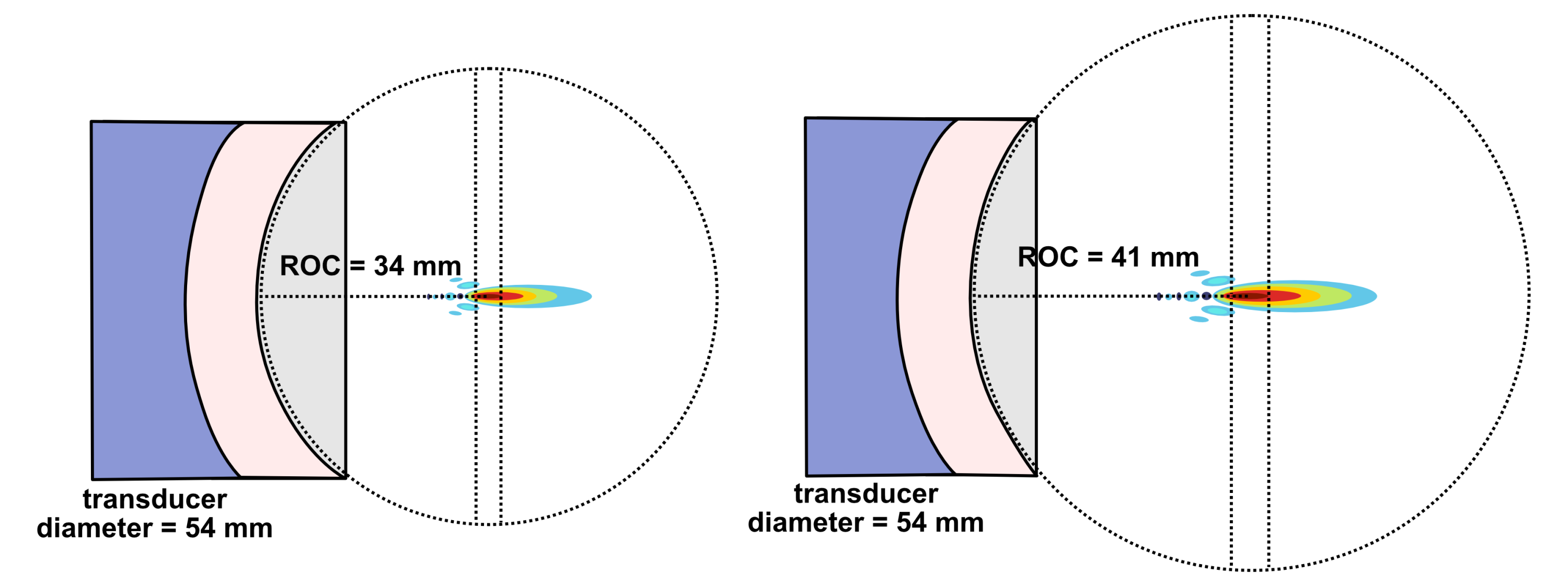
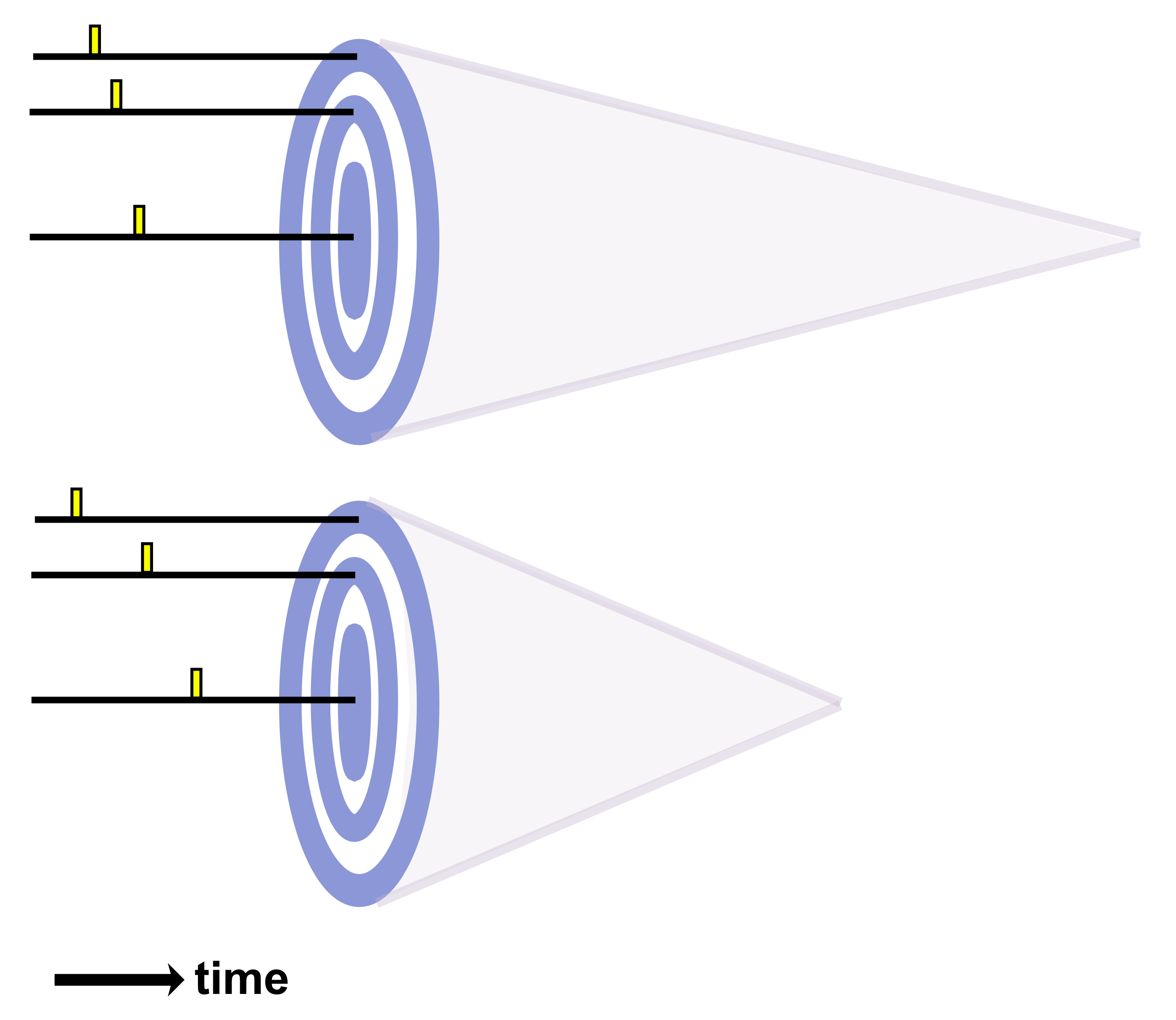
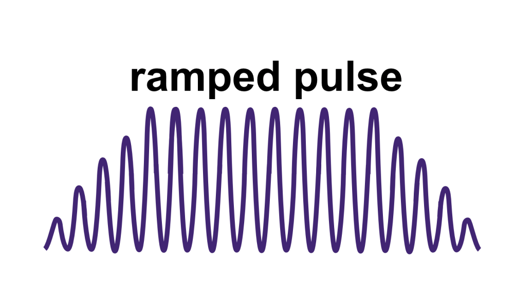
In my view, sonogenetic genes have immense potential as payloads for psychiatric gene therapy. Sonogenetics broadly speaking involves delivery of genes encoding mechanosensitive proteins, often ion channels.45 The mechanosensitive proteins change state (e.g. channel opening) in response to ultrasound waves, allowing neuromodulation through transcranial focused ultrasound (tFUS). Sonogenetic gene therapy should thus enable both millimeter-scale spatial resolution and cell-type-specific targeting for neurostimulation, offering unprecedented possibilities for treatment of psychiatric diseases.14–17 This technological convergence could radically transform how mental illness is treated. But delivery nonetheless remains among the most central challenges which must be overcome before sonogenetics reaches clinical feasibility. Neuromedicine cannot explore sonogenetic therapies without a strong foundation of enabling delivery systems.
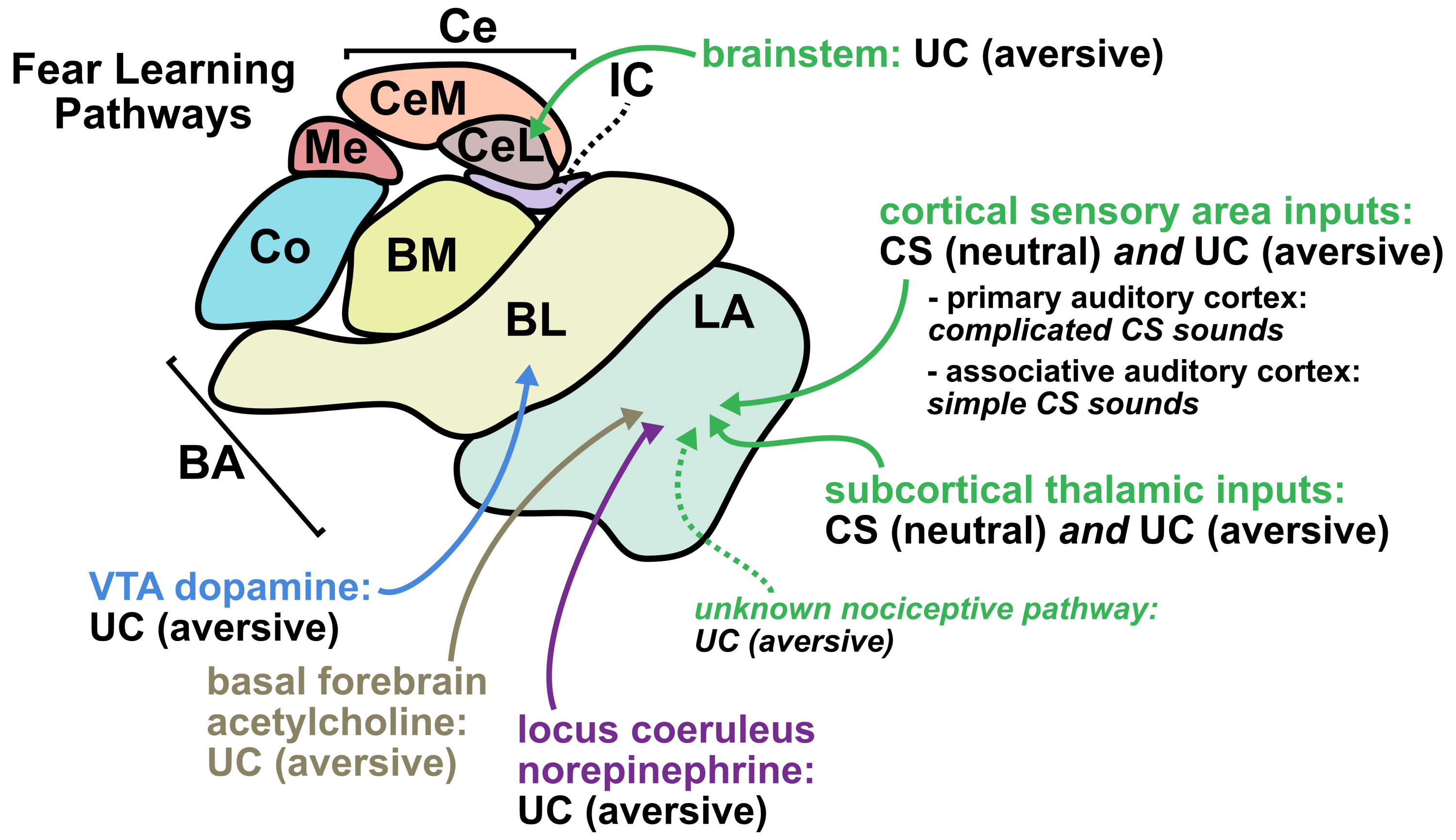
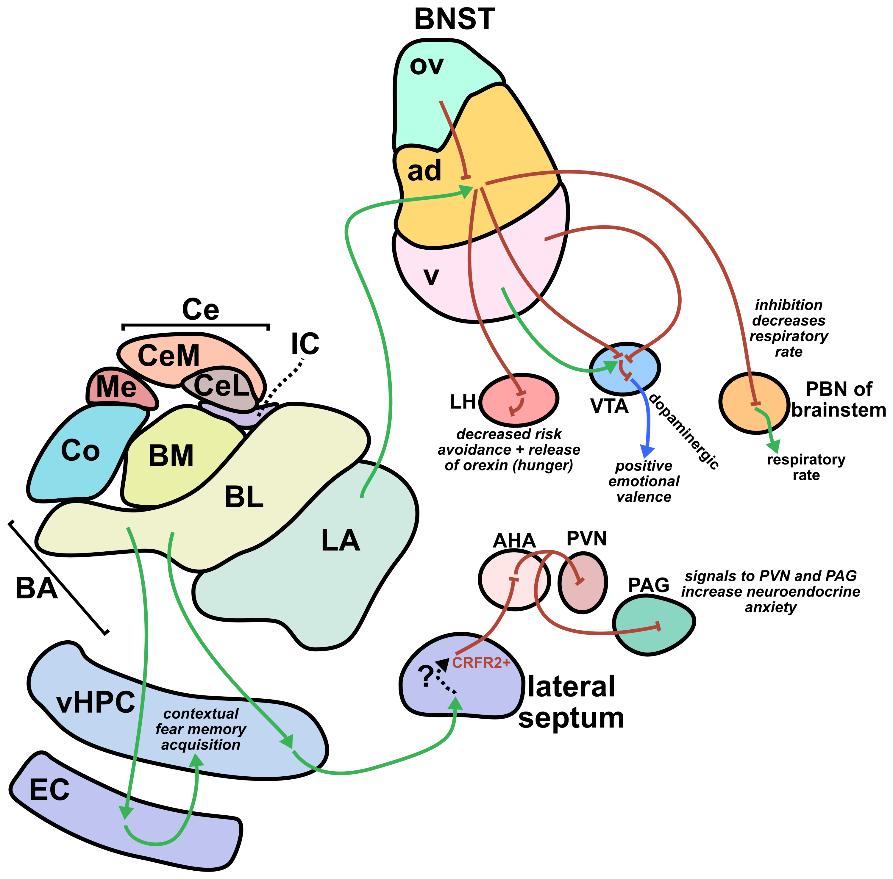
From a translational perspective, one of the greatest strengths of sonogenetics is that the different effects of stimulating a chosen neuronal cell type across numerous human brain regions may rapidly be tested. While this could have benefits at the preclinical level as well, the most important outcomes will likely occur during clinical stage testing. As an example, consider an anxiety disorder patient who has received a gene therapy which expresses mechanosensitive ion channels in a brain-wide fashion across GABAergic neurons. A clinician might leverage tFUS stimulation in the patient’s lateral amygdala for a few weeks.46,47 If that strategy did not improve the patient’s symptoms, the clinician may easily switch the tFUS stimulation to the central amygdala region46 or the bed nucleus of the stria terminalis (BNST)48 or the lateral septum.49 Many distinct brain regions could be explored without needing to develop a new therapeutic. This would allow fast clinical screening of strategies for modulating neural circuits towards better mental health. Since the challenges of clinical trials represent a massive limiting factor for therapeutics in general, the ability to quickly explore this space of possibilities could dramatically accelerate discovery. Combining the incredible precision of sonogenetic tFUS with such a rapid screening strategy may reveal superior therapeutic targets for combating mental illness.
Conclusion
As I have discussed in this essay, a lack of scalable delivery systems is a central roadblock to the promise of psychiatric gene therapy. Because of this, I have begun developing strategies for overcoming the scalable delivery problem through a number of ideas. I have done early-stage experiments towards a couple of these ideas while others remain in the ideation stage. (I cannot publicly describe the details of my ideas on the internet because public disclosure of IP precludes patentability). I should note that I am currently a graduate student and expect to complete my PhD in around six months. This article represents part of my efforts to lay the groundwork for my upcoming scalable brain delivery plans.
Mental illness represents one of the most profound challenges facing humanity. It affects how we live our lives and interact with the world. It affects people we love. It takes away precious time from people who otherwise could have been experiencing the extraordinary beauty of life and the universe. I believe that positive emotional experiences represent the most fundamental form of value in the cosmos. Mental illness blocks people off from experiencing joy, which is in my view an immeasurable tragedy that needs to be righted. It is time to do the science needed to reset our brains to live life to the fullest.
If you are interested in discussing anything related to this space, please reach out to: logan (dot) phospholipid (at) gmail (dot) com!
If you would like to read more about me and my scientific and entrepreneurial background, please check out my bio at: https://logancollinsblog.com/
References:
1. Mental disorders (World Health Organization). https://www.who.int/news-room/fact-sheets/detail/mental-disorders (2025).
2. Marx, W. et al. Major depressive disorder. Nat. Rev. Dis. Prim. 9, 44 (2023).
3. Craske, M. G. et al. Anxiety disorders. Nat. Rev. Dis. Prim. 3, 17024 (2017).
4. Leucht, S. et al. Schizophrenia. Nat. Rev. Dis. Prim. 11, 83 (2025).
5. Vieta, E. et al. Bipolar disorders. Nat. Rev. Dis. Prim. 4, 18008 (2018).
6. Yehuda, R. et al. Post-traumatic stress disorder. Nat. Rev. Dis. Prim. 1, 15057 (2015).
7. Strang, J. et al. Opioid use disorder. Nat. Rev. Dis. Prim. 6, 3 (2020).
8. MacKillop, J. et al. Hazardous drinking and alcohol use disorders. Nat. Rev. Dis. Prim. 8, 80 (2022).
9. De Brito, S. A. et al. Psychopathy. Nat. Rev. Dis. Prim. 7, 49 (2021).
10. Gunderson, J. G., Herpertz, S. C., Skodol, A. E., Torgersen, S. & Zanarini, M. C. Borderline personality disorder. Nat. Rev. Dis. Prim. 4, 18029 (2018).
11. An, S. et al. Global prevalence of suicide by latitude: A systematic review and meta-analysis. Asian J. Psychiatr. 81, 103454 (2023).
12. Hyman, S. E. Revitalizing Psychiatric Therapeutics. Neuropsychopharmacology 39, 220–229 (2014).
13. Roth, B. L. Molecular pharmacology of metabotropic receptors targeted by neuropsychiatric drugs. Nat. Struct. Mol. Biol. 26, 535–544 (2019).
14. Liu, T. et al. Sonogenetics: Recent advances and future directions. Brain Stimul. 15, 1308–1317 (2022).
15. Xian, Q. et al. Modulation of deep neural circuits with sonogenetics. Proc. Natl. Acad. Sci. 120, e2220575120 (2023).
16. Hahmann, J., Ishaqat, A., Lammers, T. & Herrmann, A. Sonogenetics for Monitoring and Modulating Biomolecular Function by Ultrasound. Angew. Chemie Int. Ed. n/a, e202317112 (2024).
17. Tang, J., Feng, M., Wang, D., Zhang, L. & Yang, K. Recent advancement of sonogenetics: A promising noninvasive cellular manipulation by ultrasound. Genes Dis. 11, 101112 (2024).
18. Miyakawa, N. et al. Chemogenetic attenuation of cortical seizures in nonhuman primates. Nat. Commun. 14, 971 (2023).
19. Bendixen, L., Jensen, T. I. & Bak, R. O. CRISPR-Cas-mediated transcriptional modulation: The therapeutic promises of CRISPRa and CRISPRi. Mol. Ther. 31, 1920–1937 (2023).
20. Doudna, J. A. The promise and challenge of therapeutic genome editing. Nature 578, 229–236 (2020).
21. Zhao, M., Zhao, Z., Koh, J.-T., Jin, T. & Franceschi, R. T. Combinatorial gene therapy for bone regeneration: Cooperative interactions between adenovirus vectors expressing bone morphogenetic proteins 2, 4, and 7. J. Cell. Biochem. 95, 1–16 (2005).
22. Won, Y.-W. et al. Synergistically Combined Gene Delivery for Enhanced VEGF Secretion and Antiapoptosis. Mol. Pharm. 10, 3676–3683 (2013).
23. Wang, J. & Vos, J.-M. H. Infectious Epstein-Barr virus vectors for episomal gene therapy. in Gene Therapy Methods (ed. Phillips, M. I. B. T.-M. in E.) vol. 346 649–660 (Academic Press, 2002).
24. Alba, R., Bosch, A. & Chillon, M. Gutless adenovirus: last-generation adenovirus for gene therapy. Gene Ther. 12, S18–S27 (2005).
25. Collins, L. T., Ponnazhagan, S. & Curiel, D. T. Synthetic Biology Design as a Paradigm Shift toward Manufacturing Affordable Adeno-Associated Virus Gene Therapies. ACS Synth. Biol. 12, 17–26 (2023).
26. Reid, C. A., Hörer, M. & Mandegar, M. A. Advancing AAV production with high-throughput screening and transcriptomics. Cell Gene Ther. Insights (2024).
27. Cameau, E., Glover, C. & Pedregal, A. Cost modelling comparison of adherent multi-trays with suspension and fixed-bed bioreactors for the manufacturing of gene therapy products. Cell Gene Ther. Insights (2020).
28. Smith, J., Grieger, J. & Samulski, J. Overcoming bottlenecks in AAV manufacturing for gene therapy. Immuno-oncology Insights (2018).
29. Gangurde, R. & Winitsky, S. Gene therapy: are high costs and manufacturing complexities impeding progress? https://www.parexel.com/insights/blog/gene-therapy-are-high-costs-and-manufacturing-complexities-impeding-progress (2024).
30. Au, H. K. E., Isalan, M. & Mielcarek, M. Gene Therapy Advances: A Meta-Analysis of AAV Usage in Clinical Settings. Front. Med. Volume 8-, (2022).
31. Huang, Q. et al. An AAV capsid reprogrammed to bind human transferrin receptor mediates brain-wide gene delivery. Science (80-. ). 384, 1220–1227 (2024).
32. Walpole, S. C. et al. The weight of nations: an estimation of adult human biomass. BMC Public Health 12, 439 (2012).
33. Gorick, C. M. et al. Applications of focused ultrasound-mediated blood-brain barrier opening. Adv. Drug Deliv. Rev. 191, 114583 (2022).
34. Batts, A. J. et al. A multifunctional theranostic ultrasound platform for remote magnetogenetics and expanded blood-brain barrier opening. Brain Stimul. Basic, Transl. Clin. Res. Neuromodulation 18, 1939–1951 (2025).
35. Nouraein, S. et al. Acoustically targeted noninvasive gene therapy in large brain volumes. Gene Ther. 31, 85–94 (2024).
36. Felix, M.-S. et al. Ultrasound-Mediated Blood-Brain Barrier Opening Improves Whole Brain Gene Delivery in Mice. Pharmaceutics vol. 13 1245 at https://doi.org/10.3390/pharmaceutics13081245 (2021).
37. McMahon, D. & Hynynen, K. Acute Inflammatory Response Following Increased Blood-Brain Barrier Permeability Induced by Focused Ultrasound is Dependent on Microbubble Dose. Theranostics 7, 3989–4000 (2017).
38. Kovacs, Z. I. et al. Disrupting the blood–brain barrier by focused ultrasound induces sterile inflammation. Proc. Natl. Acad. Sci. 114, E75–E84 (2017).
39. Patwardhan, A. et al. Safety, Efficacy and Clinical Applications of Focused Ultrasound-Mediated Blood Brain Barrier Opening in Alzheimer’s Disease: A Systematic Review. J. Prev. Alzheimer’s Dis. 11, 975–982 (2024).
40. Chen, Hong & Konofagou, Elisa E. The Size of Blood–Brain Barrier Opening Induced by Focused Ultrasound is Dictated by the Acoustic Pressure. J. Cereb. Blood Flow Metab. 34, 1197–1204 (2014).
41. Shumer-Elbaz, M. et al. Low-frequency ultrasound-mediated blood-brain barrier opening enables non-invasive lipid nanoparticle RNA delivery to glioblastoma. J. Control. Release 385, 114018 (2025).
42. Patel, D., Patel, B. & Wairkar, S. Intranasal delivery of biotechnology-based therapeutics. Drug Discov. Today 27, 103371 (2022).
43. Crowe, T. P., Greenlee, M. H. W., Kanthasamy, A. G. & Hsu, W. H. Mechanism of intranasal drug delivery directly to the brain. Life Sci. 195, 44–52 (2018).
44. Chukwu, C., Yuan, J. & Chen, H. Intranasal versus intravenous AAV delivery: A comparative analysis of brain-targeting efficiency and peripheral exposure in mice. Gene Ther. (2025) doi:10.1038/s41434-025-00585-y.
45. Legon, W. & Strohman, A. Low-intensity focused ultrasound for human neuromodulation. Nat. Rev. Methods Prim. 4, 91 (2024).
46. Babaev, O., Piletti Chatain, C. & Krueger-Burg, D. Inhibition in the amygdala anxiety circuitry. Exp. Mol. Med. 50, 1–16 (2018).
47. Benarroch, E. E. The amygdala: Functional organization and involvement in neurologic disorders. Neurology 84, 313–324 (2015).
48. Giardino, W. J. & Pomrenze, M. B. Extended Amygdala Neuropeptide Circuitry of Emotional Arousal: Waking Up on the Wrong Side of the Bed Nuclei of Stria Terminalis. Front. Behav. Neurosci. Volume 15–2021, (2021).
49. Wang, D. et al. Lateral septum-lateral hypothalamus circuit dysfunction in comorbid pain and anxiety. Mol. Psychiatry 28, 1090–1100 (2023).


")