Notes on: A Topological Representation of Branching Neuronal Morphologies, Kanari et al. 2017

Challenge

Neural morphologies involve complicated branching structures.
Traditionally, classification of such morphologies has involved qualitative assessment of microscopic images.
Topological data analysis (TDA) can classify geometric structures that are built from well-understood pieces such as spheres, cylinders, and tori. However, this sort of analysis computationally intensive when applied to neurons since their morphologies are so complex.
Feature extraction has been applied to quantitatively classify neural morphologies. This is a technique that allows a large, but potentially redundant, dataset to be converted into a reduced set of features that can be more easily analyzed.
Neurons are reconstructed as a set of points in connected by edges and then experts identify the relevant morphological characteristics to subject to the feature extraction algorithms. Unfortunately, the initial feature identification is quite subjective and can lead to different results. In addition, a great deal of information loss occurs in the processing of the data.
Neither TDA nor feature extraction are ideal for studying neural morphologies.

Topological Morphology Descriptor (TMD)

The TMD is an algorithm that maps the original images of dendritic trees to a topological representation with less information loss than other methods, though it does simplify the trees somewhat.
The TMD takes a partially ordered set of branch points (“parent” nodes with multiple further connections or “children”) and leaves (parent nodes with no further connections) as input.
Branch points and leaves are ordered by the “parent-child” relations.

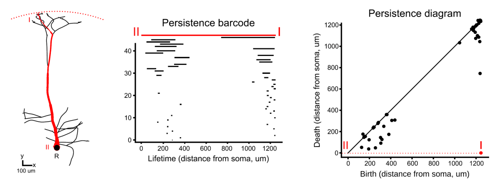
The Persistence Barcode and Persistence Diagram

This output of the TMD is a “persistence” barcode and an equivalent persistence diagram.
In the persistence barcode below (left), the distance or “lifetime” along a component (in this case a component is an individual dendritic branch) is given on the horizontal axis. This distance is measured from the component’s “birth” or most distant point from the soma to its “death” or closest point to the soma.
In the equivalent example of a persistence diagram below (right), each component’s death distance is plotted against corresponding birth distances.
Note that many possible functions f can be used to generate a persistence barcode and diagram, but here, they are ordered by lifetime with units of microns.
In the figure below, the highlighted red component is used to exemplify what an individual component looks like when analyzed in this way.

The TMD method allows analysis of any treelike structure, unlike previous techniques which were not generalizable for the various types of neural morphology. TMD is much more biologically useful and computationally inexpensive.
TMD allows a reliability measure to be assigned to proposed groupings of neuronal trees. This helps develop a diversity profile that reflects the morphological variety of neurons.

Details of the TMD Algorithm

T denotes a rooted tree embedded in (a tree with a central node or root R).
N is the set of nodes in a tree T. Furthermore, N is defined as the union of branch points B and leaves L. Individual nodes are referred to in lowercase as n
Nodes with the same parent are called siblings.
Sets of nodes are denoted as A.
Subtrees are designated T_n and centered at node n. Each subtree possesses leaves L_n. Individual leaves are .
The function f could be defined by the radial distance, the branch length, the path distance, or other characteristics. In this case, it is defined as the radial distance from the soma (or root R).
The function v (below) is computed by the TMD algorithm. It finds a maximum value for f as a function of x where x belongs to the set of leaves.

Recall that (here) f is the radial distance from the soma. As such, v(n) will find the most distant leaves.
The algorithm starts with the leaves and follows each leaf’s path down towards the soma.
Leaves are associated with their respective nodes in the set of nodes A. When a node (with one or more siblings) is encountered, all but the “oldest” sibling is removed from that node. The oldest sibling is the sibling that extends farthest from the soma. After passing through all the nodes on a particular path, the algorithm reaches the soma and designates that path as a component. The component is added to the persistence barcode.
Below are some examples of what various paths along the dendritic tree might look like. Once again, this is achieved by a process of removing the younger siblings emerging from each node along a given path.

Once all the paths have been traversed, a set of components is outputted (recall that a component is an individual branch, not the entire path). The terminus (birth) and parent node (death) of each component is known. The lifetime of each component is the distance between its birth and death. This information allows a persistence barcode and an equivalent persistence diagram to be plotted.
To reiterate, the persistence barcode and diagram describe all the individual components in a given neural tree.
The TMD algorithm has linear complexity with respect to the number of nodes.
If a tree is rotated or translated, the TMD algorithm will still give the same result.

Comparing Persistence Diagrams

There are standard topological distance measures between persistence diagrams, but this are not suited to dendritic trees. The authors defined an alternative distance measure called d_bar in the space of persistence barcodes. However, there were still issues with this metric because it converted the barcode into a one-dimensional distribution and so lost some important information for classifying neural morphologies.
The better method for comparing persistence barcodes is to convert each barcode into a matrix of pixel values (an image) by using a discretization algorithm (in this case a sum of Gaussian Kernels) and then to employ machine learning for classifying the images.