Notes on: Differential Geometry

Manifolds

Although differential geometry usually involves smooth manifolds, topological manifolds provide the foundation for understanding smooth manifolds.
Topological manifolds are a type of topological space which must satisfy the conditions of Hausdorffness, second-countability, and paracompactness (see Notes on Topology).
In addition, topological manifolds must be locally homeomorphic to Euclidean space, ℝⁿ.
In order to be locally homeomorphic to Euclidean space, the formalisms below must hold.

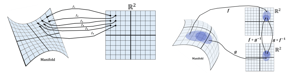
This means that, for every point x in a locally Euclidean topological space X, there exists an open set U such that x belongs to U and there exists a homeomorphism h from ℝⁿ to U (and its inverse). These homeomorphisms are called charts. The combination of charts which covers X is called an atlas.
For an atlas, two charts can overlap on a manifold. The intersection of these two charts is an open set which maps to the same region of Euclidean space. Transition maps are composition functions f(g^-1) = f∘g^-1 and g(f^-1) = g∘f^-1 which map the open sets in ℝ²to the manifold (by the inverse function) and then map back to Euclidean space (by the function which describes the other homeomorphism). This is also called a coordinate transformation.

If a manifold’s transition maps are all at least once differentiable (C¹), then the manifold is called a differentiable manifold. If the transition maps are all infinitely differentiable (C^∞), then the manifold is called a smooth manifold.

Dot products on smooth manifolds

The metric tensor allows generalization of the dot product for vectors on manifolds and is given by the equation below. Here, u and v are input vectors. The superscript and subscript indicate that uⁱ is represented as a column vector and v_j is represented as a row vector (covector to uⁱ) inside the summation. The matrix g_ij is a coefficient matrix which modifies the initial coordinate system for a given manifold. The summation is over matrix indices i and j where i=j.

To see how this equation works, consider using metric tensor to describe the dot product of two vectors in ℝ². In this case, g_ij is simply the 2×2 identity matrix.

For manifolds in general, the coefficient matrix g_ij is usually not the identity matrix. Instead, the entries of g_ij are given by the equation below involving the Jacobian matrix J.

To use this equation, new coordinates must be defined in terms of Euclidean coordinates. In order to understand this, consider the example of polar coordinates. The polar coordinate formulas are operated on by the Jacobian. When inputted into the formula for the coefficient matrix, they simplify to the result below.

Any set of alternative coordinates written in terms of Euclidean coordinates can be used to generate a g_ij matrix by this process.
An interesting application of the metric tensor is to compute the generalized dot product of two vectors on a surface (2-manifold). The vectors “start out” in ℝ², but then are mapped onto the surface, which is embedded in ℝ³. To accomplish this, the ℝ² coordinates are represented in ℝ³ by using zero for the z-components. Note that the plane is assumed to be perpendicular to the surface in this scenario.

Given a pair of vectors u and v tangent to a point on a parametric surface (2-manifold), the lengths of the vectors and the angle between them can be computed using the metric tensor. The lengths are given in the top equations and the angle is given in the bottom equations (below).

Arc lengths on smooth manifolds

The metric tensor can be used to determine the distance between the points γ(t₁) and γ(t₂) on a manifold. The vector-valued function γ(t) defines a parametric curve on the manifold. Here, g_ij is generated using the Jacobian of the parametric functions in γ(t). The components γⁱ and γ^j are equivalent when i=j since they represent the same components. The absolute value is included to keep the term under the square root positive.

Consider the example of a parametric curve in ℝ² which is mapped onto a 2-manifold embedded in ℝ³. Here, the arc length of such a curve is computed.

Integration on smooth manifolds

Integration can be performed on surfaces (2-manifolds) using surface integrals. Furthermore, this method can be generalized to volumes and hypervolumes on n-dimensional smooth manifolds.
The surface integral of a region on a 2-manifold embedded in ℝ³ can be computed by the equation below. The double-struck bars indicate magnitude. Here, the surface is given as a function z(x,y).

It should be noted that r may represent any parameterized parametrized surface (not just a surface given as z(x,y)). The more general case of a surface embedded in ℝ³ is given below.

Using some algebraic manipulations, the surface integral can be rewritten as the equation below. The matrix g represents the metric tensor (generated by applying the Jacobian to the parameterized function r).

In this form, the surface integral can easily be generalized to higher dimensions so as to integrate volumes and hypervolumes on smooth manifolds. Below, a volume integral on a smooth 3-manifold is given.