I’m writing these notes to help myself and others review mathematical probability (mostly from an applied perspective). So far, I have covered single-variable probability. I plan to later add sections on joint probability and perhaps a few other topics. My main source is the excellent textbook “Probability, Statistics, and Random Processes” by Hossein Pishro-Nik.
PDF version
Axioms of probability
The axioms of probability include: (i) for any event A, P(A) ≥ 0, (ii) the probability of the total sample space S is P(S) = 1, and (iii) if A1,A2,A3,… are disjoint events then P(A1∪A2∪A3…) = P(A1) + P(A2) + P(A3)…
Note that intersection means “and” while union means “or”. Thus P(A∩B) = P(A and B) = P(A,B) while P(A∪B) = P(A or B).
An important tool in probability is the inclusion-exclusion principle. This is given by the following formulas for two events and for n events.

Conditional probability
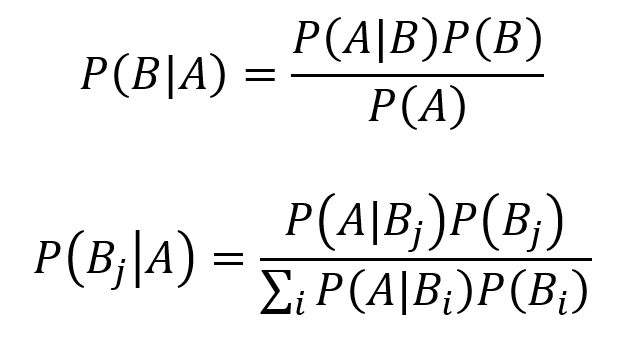
Consider two events A and B in sample space S. The conditional probability of A given B is defined by the equation below.

Two events are independent if the first equation below holds true. Three events are independent if the second, third, fourth, and fifth equations below all hold true. This logic can be combinatorically extended to n independent events as well.

The law of total probability is an important tool for working with conditional probability. If B1,B2,B3,… represents a partition of the sample space S (the sample space can be “split” or partitioned into n “regions” or disjoint sets Bi), then the law of total probability is given as follows for any event A.

Bayes theorem represents an extremely important and widely consequential tool for conditional probability. Learning the intuition behind Bayes theorem can be highly valuable. The equation for Bayes theorem with two events A and B where P(A) ≠ 0 is given by the first equation below. The equation for Bayes theorem with n events B1, B2, B3… which partition the sample space S while P(A) ≠ 0 is given by the second equation below.
Two events are conditionally independent if they satisfy the following formula.

Random variables
A random variable X is a function mapping the sample space to the real numbers. That is, X is a real-valued function that assigns a value to each possible outcome of a random experiment.
The range of X is the set of possible values for X. As an example, flip a coin 5 times and define X as the number of heads that occur. The range of X is the set RX = {0,1,2,3,4,5}.
Discrete random variables are those which have countable ranges. Examples of countable ranges include finite sets as well as countably infinite sets like ℤ, ℚ, and ℕ.
Continuous random variables are those which have uncountable ranges. Any non-empty subset of ℝ is uncountable (as is the entirety of ℝ).
Probability mass functions
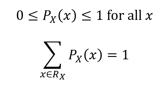
Probability mass functions (PMFs) assign probabilities to the possible values of a discrete random variable. If X is a discrete random variable with a finite or countably infinite range RX = {x1,x2,x3,…,xn}, then P(xk) = P(X = xk) for k = 1,2,3,…,n is the probability mass function of X.
As an example, the PMF for tossing a coin twice and setting X as the number of heads observed is as follows.

As it is a probability measure by definition, the PMF has the properties of a probability measure.
In addition, for any set A which is a subset of RX, the probability that X ∈ A is given as the sum of the probabilities of X for each element of A.

Independent random variables
Consider two discrete random variables X and Y. If the following equation holds true, then X and Y are independent.

X and Y are furthermore independent if knowing the probability of one of them does not alter the probabilities of the other. Note the vertical line “|” denotes “given”, so P(X =x|Y=y) is probability that X=x given that Y=y.

Special discrete distributions
Bernoulli distribution: a random variable X is a Bernoulli random variable with parameter p if its PMF is given by the first equation below. Bernoulli random variables indicate when a certain event A occurs, so they take on a value of 1 if A happens and 0 otherwise. This is described in the second equation below. Here, 0 < p < 1.

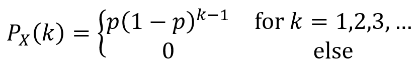
Geometric distribution: a random variable X is a geometric random variable with parameter p if its PMF is given by the equation below. The random experiment for this distribution consists of performing repeated independent “Bernoulli” trials until a given outcome (e.g. heads for a coin toss) occurs. The range of X is 1,2,3,… and describes the number of trials before the specified outcome. Here, 0 < p < 1. PX(k) tends to decline as k grows larger since it is more and more likely the specified outcome will have occurred with more trials.
Binomial distribution: a random variable X is a binomial random variable with parameters n and p if its PMF is given by the first equation below. The random experiment for this distribution consists of repeatedly (n times) performing some process which has a probability P(H) = p of yielding an outcome H, then defining X as the total number of times H is observed. Here, 0 < p < 1. Note that the binomial coefficient “n choose k” is given by the second equation below.

Poisson distribution: a random variable X is a Poisson random variable with parameter λ if its range is RX = {0,1,2,3,…} and its PMF is given by the equation below. Poisson distributions are used to describe the count of random occurrences that happen within a certain interval of time or space. For a Poisson distribution, one asks the probability that k events occur will occur within a specified interval wherein an average of λ events are known to happen.

Cumulative distribution functions
The cumulative distribution function (CDF) for a random variable X is defined by the equation below. Note that the CDF is a function over the entire real line, so it must be able to produce an output for any real input value x. An advantage of CDFs is that they can be defined for any type of random variable (discrete, continuous, or mixed).

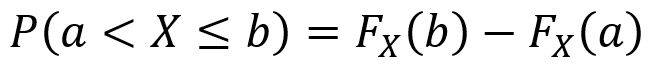
One can also use CDFs as follows to find the probability that X produces an outcome between two values a and b for which a ≤ b. Note that it is important to pay attention to when the “<” and “≤” symbols can be used.
Expectation
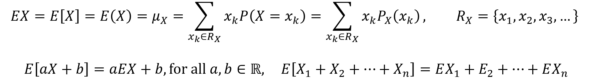
The expectation value E of a discrete random variable X is its average or mean, also described as a weighted average of the values in its range. The expectation value formula is given by the first equation below, along with various equivalent notational options. Here, the range RX of the random variable X can be finite or countably infinite. An important property of expectation is that it is linear. The linearity of expectation is described by the second equation below.
Functions of random variables
If X is a random variable and there is a function Y = g(X), then Y is also a random variable. The range of Y is RY = {g(x) | x ∈ RX} and the PMF of Y is PY(g(X) = y). A convenient way to find the expected value of E[Y] is given by the law of the unconscious statistician (LOTUS), which is described in the equation below. One can also find the PMF of Y and then use the expectation value formula, but this is usually more difficult than using LOTUS.

Variance
The variance of a random variable with mean µX is a measure of the amount of spread of its distribution. It can be found using either of the following first two equations. Some useful properties of variance are given by the second two equations.

Since variance of X has different units than X itself (variance units are the square of the units of X), standard deviation is often used as an alternative measure of distributional spread. Standard deviation is simply the square root of the variance.

Continuous random variables and probability density functions
A random variable X with a CDF of FX(x) is continuous if FX(x) is a continuous function for all x ∈ ℝ.
CDFs work properly for continuous random variables. However, PMFs are invalid for continuous random variables because P(X = x) = 0 for x ∈ ℝ when each P(X = x) corresponds to an infinitesimal slice of the probability. A different tool is needed. Specifically, the probability density function or PDF is utilized. The PDF fX(x) for a random variable X with a continuous CDF FX(x) for all x ∈ ℝ is defined by the first equation below. PDF properties are given by the rest of the equations below.

Expected value and variance for continuous random variables
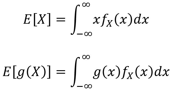
The expected value and LOTUS for continuous random variables are analogous to those in the discrete case, but with integrals instead of summations. For a continuous random variable X, the expectation value E[X] is given by the first equation below and the LOTUS is given by the second equation below.
Likewise, the variance for a continuous random variable X takes on the following equivalent forms given by the first two equations below. A useful property of continuous variance is given by the third equation below.

Finding PDFs of functions of continuous random variables
The most straightforward way to find the PDF of a continuous random variable is to start with the CDF and take its derivative (assuming the CDF is continuous).
Another way to find the PDF of a function of a continuous random variable Y = g(X) is to use the method of transformations. The simplest form of this approach requires g to be strictly increasing or strictly decreasing (a monotonic function). However, one can generalize the method of transformations by partitioning the domain RX into n intervals (where n is finite) which each are monotonic and differentiable, even if the function is not monotonic as a whole. This approach for finding the PDF is then given by the following equation.

Special continuous distributions
Uniform distribution: a continuous random variable X has a uniform distribution over the interval [a,b] if its PDF is given as follows.

Exponential distribution: a continuous random variable X has an exponential distribution with parameter λ > 0 if its PDF is given as follows.

Standard normal (standard Gaussian) distribution: a continuous random variable Z has a standard normal distribution if its PDF is given as follows (for all z ∈ ℝ). It should be noted that the standard normal distribution can be scaled and shifted to obtain other normal distributions as will be described after this discussion on the standard normal distribution.

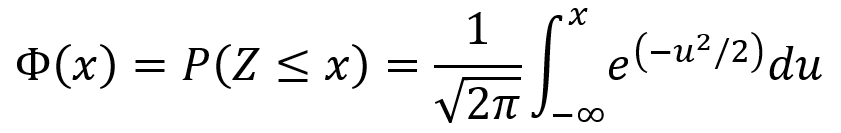
The standard normal distribution has E[Z] = 0 and Var(Z) = 1. The CDF Φ(x) of the standard normal distribution is given by the following equation.
Normal (Gaussian) distributions and normal random variables: if Z is a standard normal random variable and X = σZ + µ, then X is a normal random variable with mean µ and variance σ2. That is, X ~ N(µ,σ2). For any normal variable X with mean µ and variance σ2, the PDF is given by the first equation below and the CDF is given by the second equation below. Additionally, the probability P(a < X ≤ b) is given by the third equation below.

An important property of the normal distribution is that a linear transformation of a normal random variable is itself a normal random variable. This is described by the following theorem.

Gamma function and the Gamma distribution: the gamma distribution makes use of the gamma function, which is defined for natural numbers n = {1,2,3,…} by the first equation below and more generally for positive real numbers by the second equation below.

Some properties of the gamma function for any positive real number α > 0 are given by the five equations below.

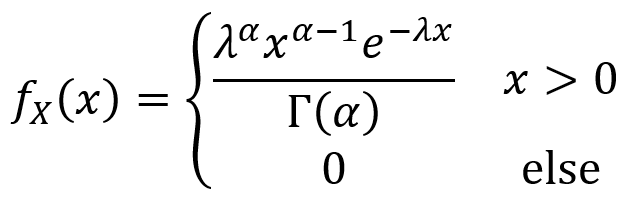
Now that the definition and properties of the gamma function have been laid out, one can move on to the gamma distribution itself. A continuous random variable X has a gamma distribution over the with parameters α > 0 and λ > 0 if its PDF is given as follows.
Mixed random variables
When a random variable contains both a continuous part and a discrete part, it is called a mixed random variable. Generally speaking, the CDF of a mixed random variable Y can be written as the sum of a continuous function C(y) and a “staircase” function D(y) as described by the equation below. The plot of FY(y) versus y can have continuous curves, discontinuities between the curves and the discrete parts. The discontinuities sometimes take the form of “jumps”.

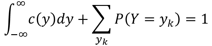
To obtain the PDF of a mixed random variable Y, one can integrate the continuous part and turn the discrete part into a sum as described by the following equation. Here, {y1,y2,y3,…} are a set of jump points of D(y). That is, they are the points for which P(Y = yk) > 0. With these mechanics, the PDF over negative infinity to infinity as well as over all jump points yk integrates and sums to 1, ensuring that the axioms of probability are satisfied.
By modifying the equation above, one can obtain the expectation value of Y as shown in the following formula.

Dirac delta function and generalized PDFs
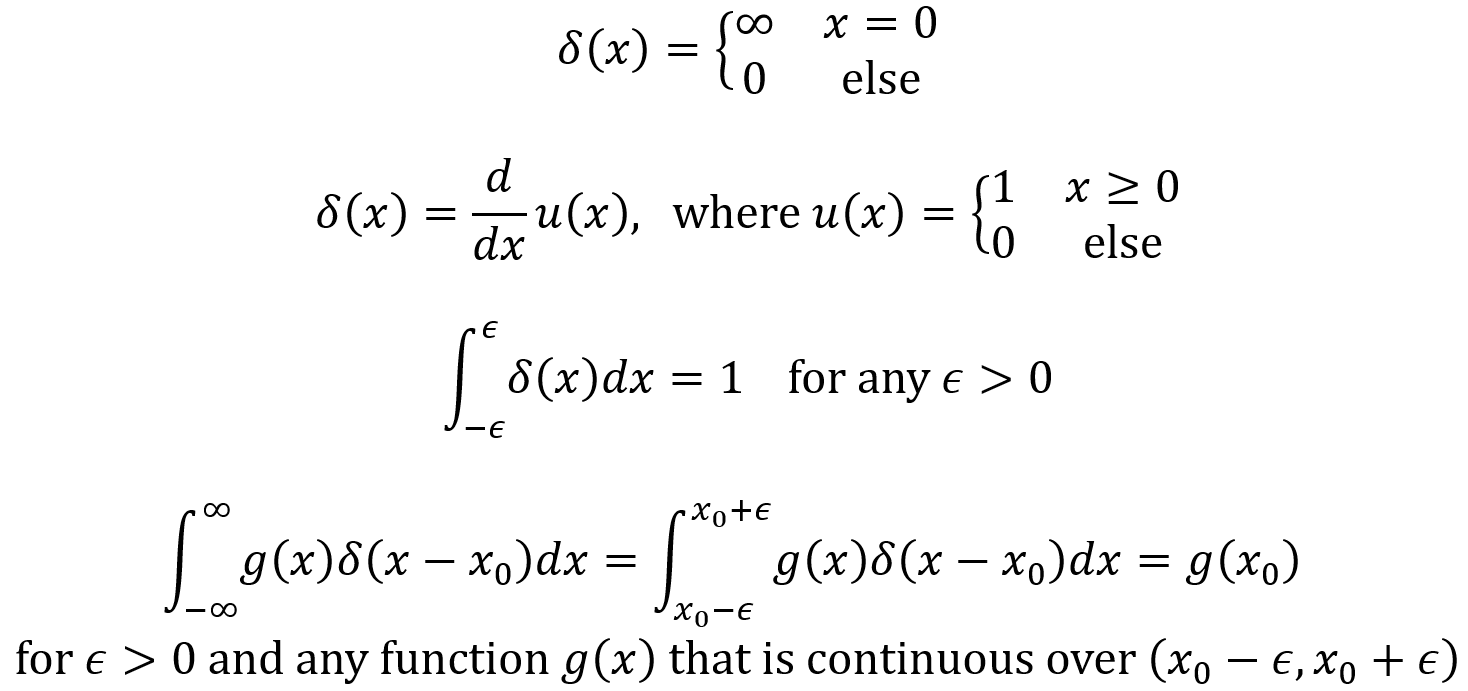
The Dirac delta function is not technically a function but a “generalized function” since it outputs an infinite value for x = 0. It is very useful since it can be used to define a PDF for discrete and mixed random variables. The Dirac Delta function δ(x) and its properties are given by the following equations. Note that u(x) is called the unit step function.
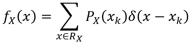
By using the Dirac delta function, one can define a generalized PDF for a discrete random variable as follow. For the random variable X here, the range RX = {x1,x2,x3,…} and the PMF is PX(xk).
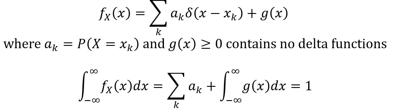
More broadly, the generalized PDF for a mixed random variable X is given by the first equation below. The second equation below describes how this generalized PDF satisfies the axioms of probability since its integral from negative infinity to infinity is 1.

One Comment