Author: logancollins

Notes on Fundraising Mechanics for Startups


No Comments

PDF version: Notes on Fundraising Mechanics for Startups by Logan Thrasher Collins

A company’s valuation is initially an estimate of how much the company is worth as set by methods such as the following.

  • Comparable transactions: looking at valuations of startups at a similar stage in the given sector.
  • Berkus method: assigning dollar values to qualitative factors such as idea, team, prototype, sales, etc. and adding them up to obtain the valuation of the company.
  • VC method: estimate the exit value of the company (value when it is sold) and divide by the firm’s desired multiple on invested capital or MOIC (e.g. 10×) to obtain the post-money valuation Vpost. Then subtract the amount invested to obtain the pre-money valuation Vpre.

Pre-money valuation is the company’s agreed-upon value before new capital is invested. It sets the price at which new shares can be sold and thus dictates how much of the company the founder gives up for the round. Post-money valuation is the pre-money valuation plus the newly invested amount of funds. It dilutes everyone’s percent ownership immediately after the round.

Dilution refers to the decrease in the percentage of the company owned by the founders. So, one might say “the round diluted us by 20%” or “we sold 20% of the company” or “the founders are at 80% ownership post-money”.

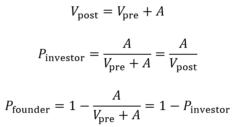
  • When raising an amount A of funds at a pre-money valuation of Vpre, the post-money valuation Vpost of the company equals Vpre + A.
  • The proportion owned by the investor Pinvestor after the round is A divided by Vpost. Multiply by 100 to obtain percentage.
  • The proportion owned by the founder Pfounder after the round is 1 – Pinvestor. Multiply by 100 to obtain percentage.

Though it can vary widely, a common dilution percentage to aim for is 20%. This allows for raising at a solid valuation while mitigating the risk of not hitting the fundraising target for the next round (and facing a “down-round”).

For a subsequent round of fundraising, the post-money valuation of its preceding round is used as a reference point for starting to evaluate the new pre-money valuation. However, it is usually not the final number. If the new pre-money valuation is higher, the round is referred to as an “up-round”. If the new pre-money valuation is the same, the round is referred to as a “flat round”. If the new pre-money valuation is lower, the round is referred to as an “down-round”.

Several factors can influence the new round’s pre-money valuation.

  • If a company hits its milestones (e.g. revenue, new data, patents, hires), this can justify a markup where the investors pay more for less dilution of the founder’s ownership.
  • If a company does not hit its milestones or grow, a flat round or down-round may be the only option to move forward.
  • Market conditions for a given industry can fluctuate and push the company’s price (pre-money valuation) up or down.
  • Other factors such as SAFEs, convertible notes, and option pool top-up can influence the company’s price.

When a company raises a priced equity round, the board and stockholders authorize the creation of shares and sell them to the investor (an issuance) if there are not enough unissued shares available. Price per share is calculated by dividing valuation V by the company’s number of shares. When new shares are issued in a round, the number of new shares is the amount A raised divided by the price per share.

Higher valuations lead to higher price per share and fewer shares issued for the same amount of investment, which means less dilution. Larger round sizes with more cash lead to more shares issued at the same price, which means more dilution.

Shares may exist as units of common stock or preferred stock. A company’s common stock is typically held by founders and employees. Unlike preferred stock, it does not come with special contractual protections. Those who hold common stock have standard voting rights for decisions like board elections, mergers, etc.

Preferred stock (usually a type called convertible preferred) is a type of equity that is typically held by investors. It comes with a number of protections for investors including liquidation preference (discussed in the next paragraph), having a separate preferred vote on major company actions, anti-dilution protections, pro rata rights (discussed in the next section), and sometimes board seats or rights to observe board meetings.

Liquidation preference describes the multiple by which the investor receives their original investment back after a liquidation event (e.g. acquisition/merger,  asset sale, winddown). Term sheets define what counts as a liquidation event. The multiple is usually 1×, but higher multiples exist (1.5×, 2×, etc.) and are not as founder-friendly.

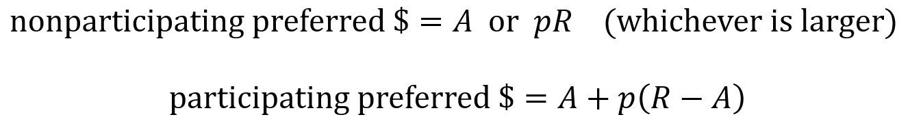
Preferred stock can be categorized as non-participating or as participating. When a liquidation event happens for a non-participating preferred stock, the investors receive their money back as either the “preference” or the “as-converted common”. The preference is the original amount they invested multiplied by the liquidation preference factor. The as-converted is the amount of money generated from the liquidation event times the percentage of the company owned by that investor.

  • For example, consider a $12M acquisition of a company where the investor originally invested $5M at a $15M pre-money valuation ($20M post-money valuation). The investor owns 25% of the company based on these numbers.
  • So, the investor can take 25% of $12M (which is $3M) or can take their original $5M back. Because $5M is higher, they receive $5M.
  • But for an example with an acquisition of $200M, the investor would take higher value of 25% of the $200M (which is $50M) rather than the original $5M.

When a liquidation event happens for a participating preferred stock, the investor first takes the preference amount (their original investment) and then takes additional funds pro rata, which here means they take an amount equal to the remaining money from the liquidation event times their percentage ownership. (Pro rata rights are discussed more in the next section).

  • Consider again the example of a $12M acquisition of a company where the investor originally invested $5M at a $15M pre-money valuation ($20M post-money valuation) and thus owns 25%.
  • The investor first takes $5M, then additionally takes 25% of the remaining $12M – $5M = $7M, where 25% of $7M = $1.75M.
  • So, the investor takes a total of $5M + $1.75M = $6.75M.

The effects of non-participating preferred and of participating preferred are summarized by the following equations where R is the amount of money from the liquidation event (the return), A is the original amount invested and p is the percentage of the company owned by the investor (as a proportion).

Pro rata rights are a legal stipulation that gives existing investors the right (but no obligation) to buy enough shares in a future financing round to retain the same ownership percentage as their initial investment. For example, if an investor owns 20% in the seed round and has pro rata rights, then they have the right to purchase 20% of new shares issued during the series A round so that they keep the same percentage ownership. (With the board’s authorization, the corporation issues new shares so that additional investment can be taken on).

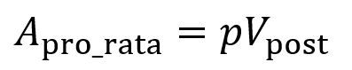
Consider an existing investor with pro rata rights and owns p% of the company before the new round. The company raises an amount of A dollars at an agreed upon post-money valuation of Vpost. For the existing investor to keep ownership of the p% of the company, they must invest an amount Apro_rata (where p is the percentage converted to a fraction).

The amount Apro_rata comes in addition to the amount invested by the new lead investor, so at least one of three items must be adjusted.

  • The round size must grow (this is most common).
  • The new lead investor’s ownership must shrink (this is rarer).
  • The valuation must increase so the lead investor still obtains their target percentage ownership.

As an example, consider a series A round (note: do not confuse “series A” with the variable A chosen to represent amount of funds invested) raised after a seed round where the seed investor was given pro rata rights.

  • In this example, let the target series A post-money valuation be $30M and new the lead investor’s target ownership be 20%.
  • Without the seed investor having pro rata rights, the lead investor would be able to invest $6M (adding to a $24M pre-money valuation) and own 20% of the company. If the seed investor’s stake is worth $4.8M (owning 20% of $24M beforehand), then the seed investor’s ownership will be diluted to 16% due to the lead investor having bought more of the company.
  • With the seed investor having pro rata, they will have the right to invest another $1.2M (buy $1.2M worth of shares) when the target post-money valuation stays at $30M, keeping them at 20% since they previously held a stake value of $4.8M (20% of $24M) and they now hold a stake value of $4.8M + $1.2M = $6M (20% of $30M).
  • With the seed investor having pro rata rights, the new lead investor will only be able to invest $4.8M (16% of $30M) assuming the post-money valuation must stay at $30M.
  • With the seed investor having pro rata rights, the lead still could invest $6M and retain 20% ownership if the post-money valuation rises to $36M or the total round amount grows to $7.2M.

An ESOP is a collection of a company’s shares that it reserves (but has not yet issued) for giving to current and future employees and advisors. It facilitates talent attraction and retention and aligns employee incentives with the company’s incentives. On cap tables, ESOP appears despite the shares not having been issued (it is labeled as “non-issued options”) and is counted when calculating ownership percentages. At the seed and series A stages, ESOPs typically occupy around 10%-15% of the cap table. Note that ESOPs are taken out of the founder’s shares and not the investor’s shares.

VCs generally require the ESOP pool to be included or “topped up” within the pre-money valuation so that dilution from the ESOP does not dilute them but instead affects the founders and earlier stakeholders.

To calculate the size of the option pool and how it affects the new investor’s shares, first find the post-money valuation Vpost from the amount invested A and the investor’s target ownership percentage.

  • For example, if the investor provides $6M and has a target ownership percentage of 20%, then the Vpost = $6M/0.2 = $30M.
  • Let x equal the number of option pool shares necessary to reach 10% at post-money valuation. Let y equal the new shares that the investor will purchase with the $6M. In this example, the number of pre-round shares will be 10M without the ESOP top-up.
  • Ownership percentages are measured after the round closes. Solving the algebraic system of equations below gives x = 1.4286M shares and y = 2.8571M shares.

  • Pre-round share count after ESOP top-up is 10M + 1.4286M = 11.4286M.
  • Number of total post-round shares is 10M + 1.4286M + 2.8571M = 14.2857M.
  • Price per share is $30M/14.2857M = $2.10.
  • Pre-money valuation is therefore 11.4286M×$2.10 = $24M.
  • The ESOP pool top-up decreases the founder’s effective pre-money valuation since the price per share falls from $24M/10M = $2.40 to $24M/11.4286M = $2.10. That is, since the founder still holds 10M shares, the founder’s stake is 10M×$2.10 = $21M (rather than $24M).

A convertible note acts as a short-term loan investors make to a startup. It is similar to debt in that it has a principal amount, interest rate, and maturity date. However, the expectation is that the note will convert into preferred equity when a later priced round is raised (e.g. a series A). Since valuation is set later, the negotiations move faster and legal fees for convertible notes remain lower.

Convertible notes come with a discount on shares for early-stage investors. (Often around 15%-25% off of the share price paid by series A investors). This rewards early investors who take a risk on the company.

Convertible notes come with a valuation cap which sets the maximum price per share once conversion to equity occurs. (For pre-clinical companies, often around $8M-20M for pre-money caps). This protects early investors if the series A price per share is high.

Convertible notes come with interest (often around 4%-8% simple interest accruing to principal) which also converts into equity upon raising a priced round. This further rewards early investors.

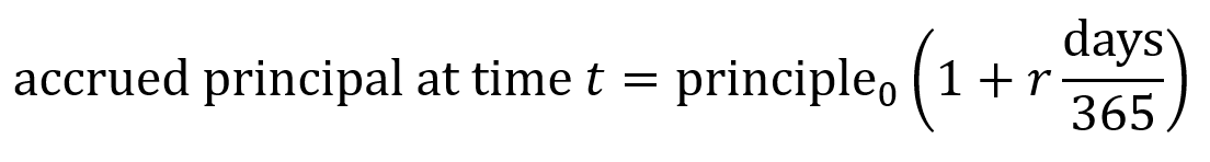
The accrued principal is the total amount that needs to be “paid back for the loan” (though in this case it will be paid back in equity) which consists of the principal (base loan amount of money) plus the accrued interest. Seed-stage biotech convertible notes usually use simple interest rather than compounding interest. Simple interest is calculated linearly using the equation below where r is the interest rate as a proportion (e.g. 6% interest = 0.06 = r). Number of days is counted from the issue date until the conversion trigger or the maturity date.

Convertible notes come with a maturity date (often around 18-36 months). If no priced round occurs by the maturity date, investors may (i) force conversion of their shares into common stock, (ii) extend the maturity date, or (iii) require repayment. Maturity dates should thus be chosen to give ample room to complete one’s next milestone.

The early investors purchase shares at a conversion price which is the lower of either the discounted series A price or the price implied by the cap.

  • As an example, consider a situation where one raises $1M on a convertible note with 6% interest, a 20% discount, and a $12M cap. In this example, let us say that there are 4M pre-money shares.
  • Eighteen months later, a series A of $20M in new capital is raised at $4.00 per share.
  • With the interest, the accrued principal amount is $1M(1 + 0.06×1.5 years) = $1.09M.
  • The discounted price per share is $4.00×(1 – 0.20) = $3.20
  • The capped price per share is $12M/(4M shares) = $3.00
  • So, the note converts at $3.00 per share price since that is the lower value between the discounted price and the capped price.
  • $1.09M/$3.00 = 363,333 new preferred stock shares issued to the note holder (the investors).

It is important to realize that the stockholders approve the board’s creation of new shares to pay back the convertible note. Everyone’s ownership percentage adjusts accordingly.

A SAFE or Simple Agreement for Future Equity is similar to a convertible note in that the investor gives a startup funding in exchange for the right to receive equity later. Unlike convertible notes, SAFEs do not accrue interest nor do they have a maturity date.

Conversion is triggered when the company raises a priced round (typically a series A). Conversion can also happen when a liquidity event occurs (e.g. acquisition or IPO). The amount of money provided by the SAFE then converts into equity, at which point the investor receives shares as determined by the valuation and number of shares issued. Investors only own shares once the conversion happens.

As protections for investors, SAFEs can (but do not always) include valuation cap, discount, and/or most favored nation (MFN) clause.

Valuation cap is the maximum post-money valuation at which the SAFE converts into equity. Even if the valuation of the company is later set at higher, the SAFE converts at the valuation set by the cap, leading to the investor receiving shares as if the cap were the valuation.

  • For example, consider a scenario where the SAFE investment is $100K, the cap is $4M the company raises a $5M series A round at a $10M pre-money valuation, and shares are priced at $1.00/share.
  • There are 10M shares initially from the $10M/($1.00/share). The series A investor adds $5M/($1.00/share) = 5M more shares. Still more shares (see below to find the exact number) are then added due to the SAFE.
  • The amount of shares from the SAFE can be calculated by first determining the SAFE holder’s percentage ownership. Divide their investment amount A by the post-money cap Cpost, so A/Cpost = 100K/4M = 2.5% ownership.
  • Next take the 2.5% ownership of the SAFE investor and divide by the total remaining percentage ownership (100% – 2.5% = 97.5%) and multiply by the initial number of shares (10M here), so 10M(2.5%/97.5%) = 256,410 shares.
  • 10M (founders) + 5M (series A investor) + 256,410 (SAFE investor) = 15,256,410 shares total.
  • In the end, the founders own 10M/15,256,410 = ~65.6%, the series A investor owns 5M/15,256,410 = ~32.8%, and the SAFE investor owns 100K/15,256,410 = ~1.68%.
  • Note that if there was no cap, the SAFE investor would receive $100K/($1.00/share) = 100K shares instead. This would correspond to $100K/($15M + $100K) = 0.66% ownership by the SAFE investor after the series A round (which is much less than with the cap).

As an interesting side note, valuation cap used to correspond to pre-money valuation, but this was changed by Y Combinator to post-money valuation in 2018. Now almost all SAFEs use post-money valuation for their calculations.

Discount means the investor receives a percentage discount (often ~10%-20%) on the share price in the round when the SAFE converts to equity. Note that this only occurs in the conversion round and does not persist into future rounds beyond that.

  • As an example, consider a scenario where the series A investor pays $1.00 per share and the SAFE has a 20% discount.
  • The SAFE then converts at $0.80 per share and the SAFE holder receives more shares for the same amount of money compared to the new series A investors.

Finally, an MFN clause gives the SAFE holder investors to adopt better terms if the company issues SAFEs later which have more favorable provisions. The original SAFE holder investors can then receive the more favorable provisions found in the terms of the new SAFEs.

Key facts about protein vault biology


No Comments

PDB 4V60: structure of a protein vault (MVP only)

Structure and organization:

Wild-type vaults consist of multiple copies of major vault protein (MVP), VPARP, and TEP1 proteins as well as small untranslated RNAs called vRNAs (Pupols, 2011).

Vaults are ~13 MDa in mass if VPARP, TEP1, and vRNAs are included along with the 78 MVPs (Galbiati et al., 2018). Each of the 78 MVP copies is ~97 kDa (Champion et al., 2009), so the hollow vault mass is ~7.7 MDa.

VPARP catalyzes poly-ADP ribosylation. It has been found to ribosylate itself and MVP. Its function is unknown. It contains the INT domain, which binds to the interior waist region of the vault (Pupols, 2011).

TEP1 (telomerase-associated protein 1) is found both associated with nuclear telomerase complexes and with cytosolic vaults. Its function is unknown (Pupols, 2011).

vRNAs are untranslated RNA polymerase III transcripts ranging from 80-150 nucleotides in length. Their function is unknown (Pupols, 2011).

Physiology and dynamics:

Vaults are found inside every cell in the human body at copy numbers of ~104 vaults per cell in most cells but ~105 in certain cell types (e.g. some immune cells) (Travis, 2024). They are especially abundant in tissues exposed to external stressors such as bronchus, renal proximal tubules, digestive tract, macrophages, and dendritic cells (Pupols, 2011). In embryonic tissues, vaults sometimes can occur at an impressive ~107 copies per cell (Suprenant, 2002).

Vaults do not self-assemble from MVP on its own. They can only be made co-translationally on eukaryotic polyribosomes (Mrazek et al., 2014). Two copies of MVP, oriented in opposite directions, are first translated by two ribosomes. The N-terminal regions of these MVPs dimerize. As more ribosome pairs arrive in line, more MVP dimers are made. Lateral interactions between the dimers begin assembling the wall of the vault. In total, 39 copies of MVP dimer are translated on the polyribosome, leading to the formation of the final barrel-shaped vault structure.

Vaults have consistently been found as contaminants in purified extracellular vesicle (EV) preparations. There is evidence that vaults associate with the outside of EVs and are not protected beneath vesicular membranes (Liu et al., 2023). However, vaults have also been found to be released from cells in an EV-independent fashion wherein they are not bound to the outside of the EVs (Jeppesen et al., 2019). As such, they might be co-released alongside EVs.

Vaults frequently exchange halves when in solution, indicating their dynamic structural nature (Yang et al., 2010). Indeed, vaults have been proposed to experience a structural “breathing” motion.

Vaults disassemble at low pH, through mechanisms of half vault separation (Goldsmith et al., 2007) and/or weakening of the lateral associations between MVP copies (Llauró et al., 2016).

Vaults are cytosolic particles, but small amounts of them associate with the nuclear membrane at nuclear pore complexes and in some cell types (e.g. U373 glioblastoma cell line) about 5% of MVP is localized to the nucleus (Slesina et al., 2005).

As MVP is a self-protein, it is usually invisible to the immune system (Champion et al., 2009). Indeed, repeated intranasal administration of vaults carrying non-immunogenic proteins like mCherry-INT does not induce anti-vault antibodies even when MVP is fused to Z peptide (an Fc-binding peptide often used to conjugate antibodies for vault targeting to specific cell types). That said, the immune system’s tolerance to vaults can be broken if vaults carrying highly immunogenic proteins like chlamydia major outer membrane protein with INT (MOMP-INT). Repeated administration of vaults carrying MOMP-INT has been shown to induce anti-MVP antibodies.

Hints at function:

MVP knockout mice are viable but have lower survival rates when challenged with Pseudomonas aeruginosa (Frascotti et al., 2021).

Vault overexpression is found in multidrug resistant cancers, but so far this seems more of a correlation than a causation. Experimentally, overexpression of vaults alone does not produce the multidrug resistant phenotype (Frascotti et al., 2021).

In neurons, vaults localize at neurite tips and along axonal and dendritic microtubule networks. Vaults can co-precipitate with cytoplasmic RNAs that are known to be translated in response to synaptic activity (Frascotti et al., 2021).

Vaults are highly conserved (Daly et al., 2013; Slinning et al., 2024). They occur in mammals, amphibians, birds, fish, sea urchins, slime molds, and more. That said, insects, plants, and fungi do not have vaults.

References:

Champion, C. I., Kickhoefer, V. A., Liu, G., Moniz, R. J., Freed, A. S., Bergmann, L. L., Vaccari, D., Raval-Fernandes, S., Chan, A. M., Rome, L. H., & Kelly, K. A. (2009). A Vault Nanoparticle Vaccine Induces Protective Mucosal Immunity. PLOS ONE, 4(4), e5409. https://doi.org/10.1371/journal.pone.0005409

Daly, T. K., Sutherland-Smith, A. J., & Penny, D. (2013). In Silico Resurrection of the Major Vault Protein Suggests It Is Ancestral in Modern Eukaryotes. Genome Biology and Evolution, 5(8), 1567–1583. https://doi.org/10.1093/gbe/evt113

Frascotti, G., Galbiati, E., Mazzucchelli, M., Pozzi, M., Salvioni, L., Vertemara, J., & Tortora, P. (2021). The Vault Nanoparticle: A Gigantic Ribonucleoprotein Assembly Involved in Diverse Physiological and Pathological Phenomena and an Ideal Nanovector for Drug Delivery and Therapy. In Cancers (Vol. 13, Issue 4). https://doi.org/10.3390/cancers13040707

Galbiati, E., Avvakumova, S., La Rocca, A., Pozzi, M., Messali, S., Magnaghi, P., Colombo, M., Prosperi, D., & Tortora, P. (2018). A fast and straightforward procedure for vault nanoparticle purification and the characterization of its endocytic uptake. Biochimica et Biophysica Acta (BBA) – General Subjects, 1862(10), 2254–2260. https://doi.org/https://doi.org/10.1016/j.bbagen.2018.07.018

Goldsmith, L. E., Yu, M., Rome, L. H., & Monbouquette, H. G. (2007). Vault Nanocapsule Dissociation into Halves Triggered at Low pH. Biochemistry, 46(10), 2865–2875. https://doi.org/10.1021/bi0606243

Jeppesen, D. K., Fenix, A. M., Franklin, J. L., Higginbotham, J. N., Zhang, Q., Zimmerman, L. J., Liebler, D. C., Ping, J., Liu, Q., Evans, R., Fissell, W. H., Patton, J. G., Rome, L. H., Burnette, D. T., & Coffey, R. J. (2019). Reassessment of Exosome Composition. Cell, 177(2), 428-445.e18. https://doi.org/10.1016/j.cell.2019.02.029

Liu, X., Nizamudeen, Z., Hill, C. J., Parmenter, C., Arkill, K. P., Lambert, D. W., & Hunt, S. (2023). Vault particles are common contaminants of extracellular vesicle preparations. BioRxiv, 2023.11.09.566362. https://doi.org/10.1101/2023.11.09.566362

Llauró, A., Guerra, P., Kant, R., Bothner, B., Verdaguer, N., & de Pablo, P. J. (2016). Decrease in pH destabilizes individual vault nanocages by weakening the inter-protein lateral interaction. Scientific Reports, 6(1), 34143. https://doi.org/10.1038/srep34143

Mrazek, J., Toso, D., Ryazantsev, S., Zhang, X., Zhou, Z. H., Fernandez, B. C., Kickhoefer, V. A., & Rome, L. H. (2014). Polyribosomes Are Molecular 3D Nanoprinters That Orchestrate the Assembly of Vault Particles. ACS Nano, 8(11), 11552–11559. https://doi.org/10.1021/nn504778h

Pupols, M. D. (2011). Packaging RNA into Vault Nanoparticles to Develop a Novel Delivery System for RNA Therapeutics. In ProQuest Dissertations and Theses. University of California, Los Angeles PP – United States — California.

Slesina, M., Inman, E. M., Rome, L. H., & Volknandt, W. (2005). Nuclear localization of the major vault protein in U373 cells. Cell and Tissue Research, 321(1), 97–104. https://doi.org/10.1007/s00441-005-1086-8

Slinning, M. S., Nthiga, T. M., Eichner, C., Khadija, S., Rome, L. H., Nilsen, F., & Dondrup, M. (2024). Major vault protein is part of an extracellular cement material in the Atlantic salmon louse (Lepeophtheirus salmonis). Scientific Reports, 14(1), 15240. https://doi.org/10.1038/s41598-024-65683-0

Suprenant, K. A. (2002). Vault Ribonucleoprotein Particles:  Sarcophagi, Gondolas, or Safety Deposit Boxes? Biochemistry, 41(49), 14447–14454. https://doi.org/10.1021/bi026747e

Travis, J. (2024). The vault guy. Science (New York, NY), 384(6700), 1058–1062.

Yang, J., Kickhoefer, V. A., Ng, B. C., Gopal, A., Bentolila, L. A., John, S., Tolbert, S. H., & Rome, L. H. (2010). Vaults Are Dynamically Unconstrained Cytoplasmic Nanoparticles Capable of Half Vault Exchange. ACS Nano, 4(12), 7229–7240. https://doi.org/10.1021/nn102051r

Notes on Ultrasound Physics and Instrumentation


No Comments

PDF version: Notes on Ultrasound Physics and Instrumentation – by Logan Thrasher Collins

Fundamentals of ultrasound waves

Sound waves such as those in ultrasound are longitudinal waves where particles oscillate backwards and forwards along the wave’s direction of propagation. This forms regions of higher (compression) and lower (rarefaction) density. Sound waves occur through the exchange of kinetic energy from molecular movement with the potential energy from elastic compression and stretching of bonds.

The speed of sound c depends on the medium. For example, in air c = 330 m/s while in water c = 1480 m/s. The frequency of a sound wave depends on the source producing it. Frequency is measured in Hertz (Hz) where 1 Hz = 1 cycle/second. Sound waves with frequencies greater than or equal to 20 kHz are referred to as ultrasound. The wavelength of a sound wave is λ = c/f. It is measured in mm (or other units of length). A sound wave’s phase describes what position the wave starts at within a cycle of oscillation and is measured in degrees or radians. Phase shifts are typically measured relative to a phase of 0° (or 0 rad). A sound wave’s amplitude corresponds to its “loudness” and describes the height of the wave’s peaks (or depth of its troughs). Cosine-based or complex exponential equations can describe sound waves in a similar way as they describe electromagnetic waves. These equations include amplitude as a coefficient, frequency as a factor multiplied by time, and phase shift as a term added to time.

Ultrasound pressure, power, and intensity

A sound wave’s excess pressure is the difference between its peak amplitude and the normal ambient pressure of the medium. When a medium is compressed, the excess pressure is positive and when it is rarified, the excess pressure is negative. In practice, the ambient pressure is often quite low and can be ignored, in which case pressure is used rather than excess pressure. Excess pressure and pressure are measured in Pascals (Pa), which are equivalent to N/m2.

When an ultrasound wave passes through a medium, it deposits energy (measured in Joules) into said medium. The rate at which a source produces this energy is the power, which is measured in Watts or J/s. An ultrasound wave’s power is unevenly distributed across the beam and often is more concentrated near the beam’s center. Intensity is a measure of the power flowing through a unit area perpendicular (or normal) to the wave’s direction of propagation and is measured in W/m2 or W/cm2. Intensity is proportional to the wave’s pressure squared (I ∝ p2).

Ultrasound and its medium

As mentioned, the medium (material) an ultrasound wave passes through determines the sound’s speed of propagation. Specifically, the material’s density and stiffness determine the speed of sound propagation. Density ρ is often measured in kg/m3. For instance, bone’s density ρbone = 1850 kg/m3 and water’s density ρwater = 1000 kg/m3 (or 1 g/cm3). Stiffness k describes how much a material resists deformation by force F. It equals the amount of pressure (stress) needed to change the thickness of a material by a given fraction and is measured in Pa. The ratio of change in thickness ΔL over original thickness L0 is called tensile strain ε. The increase (or decrease) in length of a material due to applied force is denoted ΔL = L – L0. Stress σ or fractional change in thickness is given by change in thickness divided by original thickness of the sample. Stress over strain is the elastic modulus E (also called Young’s modulus). Here, A is the cross-sectional area of a sample perpendicular to the applied force. Note that these formulas apply only for tensile stress (which induces tensile strain), the type of stress where a material is compressed or elongated.

The relationship between a sound wave’s speed and the properties of density and thickness can be modeled by masses on springs where ρ = m = density (corresponding to masses in the model) and k = stiffness (corresponding to the spring stiffness in the model). The relationship between c, ρ, and k is given by the following equation.

As a result of these properties, the speed of sound varies in different tissues. A table of the approximate speeds of sound across selected tissues is provided.

Acoustic impedance z measures the response of a medium’s particles in terms of their velocity v to a sound wave of a given pressure p. Acoustic impedance can also be expressed in terms of density and stiffness or in terms of density and the sound’s speed. The latter form of definition is called the characteristic acoustic impedance of the tissue. It has units of kg m–2 s–1, also called rayl.

Ultrasound reflection and refraction

When an ultrasound wave traveling through a medium of acoustic impedance z1 encounters a new medium of different acoustic impedance z2, some of the wave is transmitted and some is reflected back. The equations in the following discussion will initially assume that the wave approaches the interface at a 90° angle (perpendicular) until stated otherwise.

To maintain continuity across the interface, the following equations must hold. Here, pi and vi are initial pressure and velocity, pr and vr are reflected pressure and velocity, and pt and vt are transmitted pressure and velocity.

Additionally, the intensity transmitted It across the interface equals the incident intensity Ii minus the reflected intensity Ir.

By using the equation for the definition of acoustic impedance z = p/v, the following two equations are true. Algebraically manipulating these equations leads to the third equation below. Rp is called the amplitude (or pressure) reflection coefficient of the interface. It is important because it decides the amplitude of the echoes produced at various interfaces within the tissue.

Note that if the acoustic impedance of the first medium is greater than the acoustic impedance of the second medium (i.e. z1 > z2), then Rp is negative and the reflected wave is inverted (across the x axis). For most interfaces between soft tissues, Rp is quite small and so most of the wave is transmitted to produce further echoes deeper within the tissue. This is useful for ultrasound imaging. Since the interface between air and soft tissue has a much larger Rp, the ultrasound source must be placed in direct contact with the patient’s skin to avoid air blocking transmission. This also means that gas-containing tissues like lungs and gut effectively block imaging beyond the region with the gas.

Another way to describe reflection is in terms of the intensity reflection coefficient RI. Since I ∝ p2, this means that RI = Rp2.

Since the incident intensity is Ii = It + Ir and the transmitted intensity is It = Ii – Ir, one can also define an intensity transmission coefficient TI as the first equation below. Since the transmitted pressure is pt = pi + pr, one can also define a pressure transmission coefficient Tp as the second equation below.

It is useful to realize that, because energy at interfaces must be conserved, the following equation holds true.

But ultrasound waves often do not approach interfaces at a 90° angle, so the equations in this section must be modified via trigonometry to account for other angles. First, note that the incident angle θi will equal the backscattered angle θr (this is true in the 90° case as well).

When a sound wave in a less dense tissue (slower sound wave) crosses into a tissue of greater density (faster sound wave), the transmitted wave bends away from the normal and thus θt > θi

Likewise, when a sound wave in a tissue of greater density (faster sound wave) crosses into a tissue of less density (slower sound wave), the transmitted wave bends towards the normal and thus θt < θi.

Ultrasound scattering

When ultrasound encounters an object which is small compared to the wavelength, it scatters in all directions, though slightly more energy is typically backscattered towards the transducer than away from it. Scattering specifics depend on the shape, size, and acoustic properties (z, k, ρ) of the object.

When many similar small objects are close together (e.g. red blood cells), constructive interference can occur, which is useful. In the case of the blood, this is the basis for Doppler ultrasound, which measures blood flow. By comparison, when many small objects are far apart, complex interference patterns occur. This leads to a phenomenon in images known as “speckle”, which is usually (but not always) considered a form of undesirable noise.

Absorption and relaxation of ultrasound

As ultrasound moves through tissue, it loses energy due to absorption, resulting in heat. There are two ways this occurs: relaxation absorption and classical absorption. The effects of relaxation absorption are typically much more dominant.

Relaxation absorption depends on the elastic properties of tissue, occurring when the tissue returns to its original state after rarefaction or compression by ultrasound. This is quantified by the relaxation time τ = 1/fr, which is how long the tissue takes to return to its original state after the ultrasound’s effect. 

Relaxation is characterized by a relaxation absorption coefficient βr which is given by the first two equations below. Here, fr is the frequency of relaxation, f is the frequency of ultrasound, and B0 is a material-specific constant. In practice, tissues contain a range of values of τ and fr, so the third equation below is a more general formula where the overall relaxation absorption coefficient is proportional to the sum of the various contributions. Higher values of βr mean more energy is absorbed into the tissue.

It is useful to note that in tissues, the relationship between the relaxation absorption coefficient βr and the frequency f is approximately linear.

Classical absorption is less important in tissues since, at clinical frequencies, the relaxation absorption is strongly dominant as mentioned. That said, overall absorption does consist of a combination of relaxation and classical absorption (though the latter may be approximated away sometimes). Classical absorption occurs because of friction between particles as they are displaced by ultrasound, causing loss of energy to heat. This loss is characterized by the classical absorption coefficient βclass ∝ f2.

Attenuation coefficients

When an ultrasound beam propagates through tissue, the sum of the absorption and scattering is described as attenuation, which causes an exponential decrease in the pressure and intensity of the ultrasound as a function of the propagation distance x through tissue.

The following equations describe the loss of ultrasound intensity and pressure as the wave moves through tissue. Here, µ is the intensity attenuation coefficient and α is the pressure attenuation coefficient. The value of µ is equal to twice the value of α (so, µ = 2α). Both have units of cm–1, though the value of µ is often given in units of decibels (dB) per cm, where the conversion factor is µ(dB cm–1) = 4.343µ(cm–1). It is useful to note that each 3 dB decrease corresponds to a decrease in intensity by a factor of 2.

Approximate frequency dependences of µ are given in the table below. As an example, in soft tissue, the value of µ = 1 dB cm–1 for 1 MHz ultrasound and µ = 2 dB cm–1 for 2 MHz ultrasound. Note that the value of µ for fat is calculated differently than the others via the equation µ(f) = 0.7f1.5 dB.

Ultrasound transducers

Ultrasound imaging is performed using ultrasound transducers. A gated frequency generator first produces short periodic voltage pulses, which are then amplified and fed into the transducer via a transmit-receive switch. Because the transducer transmits high power pulses and receives low intensity signals from the reflected ultrasound waves, the transmit and receive circuits must be isolated from each other. Amplified voltage is converted by a shaped piezoelectric material (typically lead zirconate titanate, which is abbreviated PZT) in the transducer into a mechanical pressure wave which is transmitted into the tissue. 

After reflecting and scattering from boundaries within the tissue, pressure wave signals return to the transducer and are converted back into voltages by the piezoelectric material. The voltages must pass through low-noise preamplifier before digitization. Further amplification and signal processing facilitates display of images on a computer.

When oscillating voltage is applied to one end of shaped PZT material, the thickness of the PZT element oscillates at the same frequency as the voltage. By placing this element in contact with skin, mechanical pressure waves are transmitted into tissue. The element has a resonant frequency f0 which is determined by its thickness T and the speed of the ultrasound wave in the PZT material cPZT. The value of cPZT is ~4000 m/s.

For most ultrasound devices, the transducer element’s thickness must be designed to equal one half the wavelength of ultrasound in the PZT material λPZT, so T = λPZT/2. This facilitates use of the resonant frequency.

Because of the much higher acoustic impedance of PZT material compared to skin (~18 times higher), a large amount of the energy would be reflected if the PZT was placed directly onto the skin’s surface. This would mean the mechanical wave traveling into the tissue would lose most of its energy.

To prevent this energy loss from happening, transducers possess a matching layer with a zmatching value between zskin and zPZT as given by the equation below. The thickness of the matching layer is typically made to be 1/4 of the ultrasound’s wavelength in its material T = λmatching/4. All this improves the transmission and reception efficiency. Sometimes multiple matching layers are used to further improve efficiency.

At the back of a PZT element, there is a damping layer, typically made of some backing material and epoxy. This damping layer prevents the PZT from continuing to oscillate (at a decaying rate) after each voltage pulse. This continued oscillation would blur the boundaries between the short pulses, which can decrease axial resolution (as will be described soon).

Although transducers have a central frequency f0, they typically cover a range of frequencies (e.g. a 3 MHz transducer might cover a range of 1-5 MHz). Higher mechanical damping leads to broader transducer bandwidth. Transducer bandwidth is described as the frequency range over which the sensitivity is greater than half the maximum sensitivity level. The relationship between bandwidth and f0 is often quantified by the quality factor Q, which is the ratio of f0 to the bandwidth. Low values of Q mean larger bandwidths. Note that 2f0 is the second harmonic frequency.

Beam geometry and resolution

FUS transducers produce a very complicated wave pattern close to the face of the transducer (the near-field or Fresnel zone). This complicated pattern is not usually useful since it has many parts where the intensity is zero. Beyond the near-field zone, the wave pattern is much simpler and decays exponentially with distance (the far-field or Fraunhofer zone). The boundary between the two zones is called the near-field boundary (NFB) and occurs at a distance ZNFB away from the face of the transducer. The following equation (where r is the radius of the transducer) can be used to calculate the ZNFB value.

After the NFB, the FUS beam diverges (spreads out laterally) with an angle of deviation θ which is given by the equation below.

For the far-field zone, the lateral shape of the beam approximates a Gaussian function. The full width at half maximum (FWHM) defines the lateral resolution of the beam. It is given by the equation below, where σ is the standard deviation of the Gaussian. This value is unique to each FUS beam at the specific desired depth. It can be calculated by the following equation.

Single element transducers also produce ultrasound side lobes where the first zero of the side lobe at angle φ is the same equation as the FUS beam’s divergence angle equation. In ultrasound imaging, the side lobes can cause artifacts if they are backscattered from tissue outside of the imaged region.

Axial resolution is the closest distance two boundaries can be relative to each other (in a direction parallel to the FUS beam’s propagation) while still allowing them to be resolved as two distinct features. It is given by the equation below where pd is the pulse duration and c represents the speed of the ultrasound in the tissue.

The reason that axial resolution works this way is because the echoes of beams returning from two different boundaries are distinguishable so long as these boundaries are spaced widely enough that they do not overlap in time.

Some typical values of axial resolution are 1.5 mm at a frequency (1/c) of 1 MHz or 0.3 mm at a frequency of 5 MHz. But it should be noted that attenuation of the FUS increases at higher frequencies, so there is an important tradeoff between penetration depth and axial resolution. (Very high frequencies such as 40 MHz can be used for imaging the skin at high resolution).

Single flat ultrasound transducers possess relatively poor lateral resolution. Concave curved transducers can achieve better resolutions. (It should be noted that the transducer equations above may be somewhat altered in the case of curved transducers rather than flat transducers). To make a curved transducer, one can add a curved plastic lens in front of the piezoelectric element or the piezoelectric element itself can be made in a concave curved shape.

The shape of a transducer’s curvature can be described by an “f-number”, which is a value equal to the focal distance divided by the aperture dimension where the aperture dimension is determined by the size of the transducer element.

Lateral resolution for a bowl-shaped curved (focused) transducer is calculated using the following equation below where λ is the ultrasound wavelength, F is the focal distance, and D is the diameter of the transducer. The focal distance F is where the lateral beamwidth is narrowest and is approximated as the radius of curvature (ROC) of the lens or PZT element. This approximation is valid except in the case of very high curvature.

When deciding on the focusing power of a transducer, there is a compromise between high spatial resolution and depth over which good spatial resolution is achievable. For a strongly focused transducer, locations further away from the beam’s focal plane diverge more sharply than for a weakly focused transducer. This can be quantified by the on-axis depth-of-focus (DOF) which equals the axial distance over which the beam’s intensity is at least 50% of its maximum value.

Transducer arrays

Contemporary FUS systems typically use arrays consisting of many small piezoelectric elements (rather than single-element transducers). These arrays allow 2D imaging via electronic steering of the beam through tissue while the transducer is held at a fixed position. Sophisticated electronics produce a dynamically changing focus during pulse transmission and signal reception, which maintains high resolution throughout the image. Linear and phased array transducers represent the two main types of arrays.

A linear array consists of many (often 128-512) rectangular piezoelectric elements where the space between elements is called kerf and the distance between their centers is referred to as pitch. Each element is mechanically and electrically isolated from its neighbors by filling the kerf regions with acoustically isolating material. The elements are not focused. Pitch is designed to range from λ/2 to 3λ/2 (where λ is ultrasound wavelength in tissue). Linear arrays are usually about 1 cm wide and 10-15 cm long.

Linear arrays work by using separate voltage pulses to excite a small number of elements at slightly different times where the outer elements are excited first and the inner elements are excited after a short delay. This creates an effectively curved wavefront with a focal point at a certain distance from the array. After all backscattered echoes have been received, another beam consisting of a distinct subset of elements performs the same steps. This is repeated in sequence until all of the groups of elements have completed the procedure. If even numbers of elements were used for each group, the entire process can be repeated again with odd numbers of elements to cover the focal points between those acquired before.

Linear array focusing occurs only in one dimension. By contrast, the elevation plane (the direction perpendicular to the image plane) cannot be focused unless a curved lens is included to produce focus in this dimension. Linear arrays are most often used for applications involving large fields of view and relatively low penetration depth.

Phased arrays are typically around 1-3 cm in length and 1 cm in width. They are used in applications like cardiac imaging where there is only a small region of the body through which the ultrasound can enter without running into bone or air.

As with linear arrays, phased arrays apply voltage pulses at slightly varying times to excite elements and produce an effective wavefront with a certain focal length. But phased arrays must employ beam steering to reconstruct a full 2D image. This occurs by changing the pattern of excitation to sweep the effective wavefront beam across a range of directions to cover the image plane.

Phased arrays also employ a process called dynamic focusing to optimize lateral resolution over the full depth of imaged tissue. This involves dynamically changing the number of elements used to produce a wavefront with varying focal lengths. At deeper regions in the tissue, the number of elements needed to position the focus (where optimal lateral resolution is achieved) is higher than at shallower regions in the tissue. Dynamic focusing allows high lateral resolution across the full depth of the scan. However, dynamic focusing is relatively slow since multiple scans are needed to build up a single line of the image. It should be noted that the length of each element determines the “slice thickness” for the image’s elevation dimension.

There are also multidimensional transducer arrays which include extra rows of transducer elements. These multidimensional arrays can focus in the elevation dimension without the need for curved elements or lenses (though they are more complicated devices). Multidimensional arrays with a small number of extra rows (e.g. 3-10) are referred to as 1.5 dimensional arrays. These 1.5D arrays can facilitate some level of focusing in the elevation dimension, though to a limited extent. When multidimensional arrays possess a large number of extra rows (up to the number of elements in each row), they are referred to as 2 dimensional arrays. These can acquire full 3D image data without needing to be moved from their initial position.

Annular arrays represent another class of transducer array. They are useful at very high frequencies (>20 MHz) since linear or phased arrays are quite difficult to create for these frequencies. Annular arrays consist of concentric rings of piezoelectric material alternating with rings acoustically isolating material. Beam forming is accomplished using an analogous strategy to that of phased arrays. The outermost rings are excited first and the innermost rings last, producing an effective focus. Because annular arrays require mechanical motion to sweep the beam through tissue for reconstruction of images, commercially available devices have been developed to precisely control this motion.

When transducer arrays receive signals, they pass through an amplifier to strengthen them before digitization. However, such amplifiers do not provide linear gain for signals with a dynamic range that exceeds 40-50 dB. This is an issue because very strong signals appear from tissue boundaries near the transducer while much weaker signals appear from tissue boundaries deeper in the body. Weak signals can thus be lost when attempting to receive over larger dynamic ranges. A process called time-gain compensation (TGC) is employed to circumvent this issue. TGC increases the amplification factor as a function of time after transmission of an ultrasound pulse. As a result, the weaker backscattered echoes which come later are amplified to a greater degree than the stronger backscattered echoes which come sooner. TGC is controlled by the operator of the instrument, which usually comes with a variety of preset values for clinical imaging protocols.

Parameters for focused ultrasound in practice

There is no universally accepted definition of FUS dose, so various metrics of exposure are used to quantify how much ultrasound is delivered during a therapeutic session. Examples of such metrics (which will be discussed further below) include acoustic pressure or peak negative pressure, mechanical index, frequency, pulse repetition frequency (PRF), and intensity.

Peak negative pressure is often measured in MPa and describes the degree of rarefaction caused by the ultrasound wave in tissue. For low intensity focused ultrasound (LIFU), the greatest mechanical safety risk is from cavitation (bubble formation and collapse). To measure cavitation risk, the mechanical index (MI) is used. MI can be computed using the following equation where Pn is the peak negative pressure, f0 is the fundamental frequency, and the derating constant of 0.3 adjusts for tissue attenuation (~7% loss per cm per MHz) and has units dBcm–1MHz–1. After derating, 0.3Pn has units of MPa. FDA guidelines specify that MI should not exceed 1.9. MI itself is unitless.

An ultrasound wave’s pulse’s duration (PD) is the number of cycles divided by the frequency. For instance, a pulse with 500 cycles of 500 kHz ultrasound would last for 1 ms. The pulse repetition interval (PRI) is the amount of time between the start of one pulse and the start of the next pulse (so it includes both the pulse and the pause after the pulse). Pulse repetition rate (PRR) also known as the pulse repetition frequency (PRF) equals 1/PRI. The pulse duty cycle (PDC) equals PD/PRI and is expressed as a percentage. PD typically ranges from microseconds to seconds, PRI from milliseconds to seconds, and PDC from <1% up to 70%.

One’s choice of a particular PD and PDC comes from two main factors: (i) the duty cycle can have varying neuromodulatory effects (excitatory or inhibitory) depending on its value and (ii) lower PDC values can be leveraged to limit total energy and heat deposition.

A pulse train is a series of pulses, for which the pulse train duration (PTD) equals the total number of pulses times the PRI. Typical PTDs range from less than 1 second to several minutes. The amount of time between the start of one pulse train and the start of the next is called the pulse train repetition interval (PTRI). The amount of time between pulse trains is called the interstimulus interval (ISI). The pulse train duty cycle (PTDC) equals PTD/PTRI.

It should be noted that the PTDC does not have a major influence on neuromodulatory effect, so the ratio is driven by safety such that the ISI is long enough to limit cumulative heating to reasonable levels.

Multiplying PDC by PTDC gives an overall duty cycle equal to (PD/PRI)(PTD/PTRI) which can be further multiplied by the average intensity of the pulses Iavg to obtain average temporal intensity Iavg_tp. FDA diagnostic safety guidelines state that average intensity should fall below 720 mW/cm2. So, Iavg_tp = (PD/PRI)(PTD/PTRI)Iavg generally should not exceed 720 mW/cm2.

Total ultrasound application time is the sum of the durations of all pulse trains plus ISIs. It typically ranges from less than 1 minute to over 60 minutes. Longer total ultrasound application time is thought to usually improve efficacy by depositing more energy, though this may not always be true. Energy per unit time might play a more significant role in efficacy, but this is an ongoing area of investigation.

Frequency (or fundamental frequency f0) is the primary frequency of FUS passing through the tissue. It is typically measured in kilohertz (kHz) or megahertz (MHz). In human neuromodulation applications, frequency typically ranges from 200-700 kHz (or 0.2-0.7 MHz), providing an acceptable tradeoff between amount of energy entering the brain and the size of the focal region. The reason that the upper limit of frequency for human neuromodulation is typically ~700 kHz is because FUS energy attenuation by the skull at 700 kHz is ~75% (though this varies depending on skull morphology) and keeps increasing at higher frequencies.

Recall from the equations in the earlier discussion that lateral resolution involves wavelength λ (and f = c/λ), so frequency influences the focal region’s size. Also discussed earlier, frequency influences the distance from the transducer to the near-field boundary (ZNFB). Frequency itself is generally not believed to contribute to neuromodulatory effects in a direct fashion, though this is still under investigation. So, the f0 value is usually selected to create a focal volume of a desired size at a given depth.

Intensity is defined as power per unit area (and recall the unit of power is Watts or J/s) and is the rate at which energy is transferred by the FUS wave. For ultrasound at any given point in time during the wave cycle, intensity is proportional to the square of the acoustic pressure as described by the equation below where P is the acoustic pressure, ρ is the density of the medium, and c is the ultrasound speed in the medium. Recall that ρc = z, the acoustic impedance. Acoustic intensity is usually measured in watts per square centimeter (W/cm2).

Beyond instantaneous intensity, FUS is often measured by spatial peak pulse average intensity (ISPPA) and by spatial peak temporal average intensity (ISPTA). ISPPA is the average intensity experienced during a single ultrasound pulse. Note that I does not equal Pn2/2z in the case of a ramped pulse. To determine average intensity (ISPPA) for ramped pulses, the integral of intensity across the pulse is divided by the pulse’s duration PD. Ramped pulses distribute energy more smoothly and help mitigate auditory confounds for LIFU applications.

ISPTA represents the average intensity of the FUS beam at the point where it is strongest averaged over the pulse duration while accounting for any off periods. It is described by the following equation consisting of the ISPPA multiplied by the PDC (which is the fraction of PRI that the pulse is turned on).

References:

1.      Legon, W. & Strohman, A. Low-intensity focused ultrasound for human neuromodulation. Nat. Rev. Methods Prim. 4, 91 (2024).

2.      Smith, N. B. & Webb, A. Introduction to Medical Imaging: Physics, Engineering and Clinical Applications. (Cambridge University Press, 2010).

Reexamining the neurobiological correlates of subjective experience for whole-brain emulation (slides)


No Comments

I presented these slides (PDF and images below) during the Workshop on Philosophy and Ethics of Brain Emulation (January 28th-29th, 2025) at the Mimir Center for Long Term Futures Research in Stockholm, Sweden. In my talk, I explored how various biological phenomena beyond standard neuronal electrophysiology may exert noticeable effects on the computations underlying subjective experiences. I emphasized the importance of the large range of timescales that such phenomena operate over (milliseconds to years). If we are to create emulations which think and feel like human beings, we must carefully consider the numerous tunable regulatory mechanisms the brain uses to enhance the complexity of its computational repertoire. At the workshop, we also discussed how the peripheral nervous system, enteric nervous system, endocrine system, musculoskeletal system, sensory systems, and perhaps even immune system may or may not play roles in subjective experience. To better understand what is needed to support proper emulations, I recommend recruitment of more fundamental neurobiology specialists to the whole-brain emulation community.

PDF: Reexamining the neurobiological correlates of subjective experience for whole-brain emulation

My abstract:

How much biological detail must a whole-brain emulation (WBE) incorporate to accurately preserve human subjective experience such that living as a WBE would truly feel like existing as a human? I ask this question independently of whether a nonbiological substrate can support subjective experience. Sandberg and Bostrom’s whitepaper Whole Brain Emulation: A Roadmap, briefly explores how levels of emulation detail ranging from abstract brain modules to quantum interactions between molecules may influence success criteria. They estimate that the necessary detail may at most involve an emulation of a connectome with multicompartmental models of neurons, dynamical synaptic states, and concentrations of metabolites and neurotransmitters in each compartment. For simplicity, I will refer to this as a multicompartmental emulation.

Although a multicompartmental emulation might produce an approximation of a human mind, I argue that the lack of additional biological layers of regulation could result in a subjective experience which has significant inaccuracies or missing pieces. Biological systems possess a massive number of tunable regulatory phenomena extending beyond multicompartmental electrophysiology. Some of these phenomena include but are not limited to morphological plasticity of brain cells, glial influence on computation, neurovascular coupling, adult neurogenesis, intercellular RNA transport, gap junctions, volume transmission, influence of perineuronal nets and other extracellular matrix (ECM) components, mechanical influences (e.g. crowding of synapses) on neuronal computation, ephaptic coupling, temporal evolution of genomic-transcriptomic state, and co-transmission of multiple neurotransmitters from the same synaptic bouton. In particular, experiences which depend on long-timescale changes across the brain may not be properly captured by a model which focuses on the fast electrophysiological dynamics of multicompartmental models with fixed connectomic and morphological properties.

To move towards accurately reproducing the feeling of humanness, I propose a first step of rigorously surveying neuroscience literature and evaluating how biological regulatory phenomena contribute to subjectively observed conscious experiences. This may facilitate construction of a draft catalogue where putative links between aspects of conscious experience and neurobiological phenomena can be established. Such an examination of the neural correlates of subjective experiences may serve as an initial guide for future efforts towards WBEs which preserve the feeling of humanness.