PDF version: Notes on Quantum Mechanics – By Logan Thrasher Collins
The Schrödinger equation and wave functions
Overview of the Schrödinger equation and wave functions
Quantum mechanical systems are described in terms of wave functions Ψ(x,y,z,t). Unlike classical functions of motion, wave functions determine the probability that a given particle may occur in some region. The way that this is achieved involves integration and will be discussed later in these notes.
To find a wave function, one must solve the Schrödinger equation for the system in question. There are time-dependent and time-independent versions of the Schrödinger equation. The time-dependent version is given in 1D and 3D by the first pair of equations below and the time-independent version is given in 1D and 3D by the second pair of equations below. Here, ћ is h/2π (and h is Planck’s constant), V is the particle’s potential energy, E is the particle’s total energy, Ψ is a time dependent wave function, ψ is a time-independent wave function, and m is the mass of the particle. After this point, these notes will focus on 1D cases unless otherwise specified (it will often be relatively straightforward to extrapolate to the 3D case).

For a wave function to make physical sense, it needs to satisfy the constraint that its integral from –∞ to ∞ must equal 1. This reflects the probabilistic nature of quantum mechanics; the probability that a particle may be found anywhere in space must be 1. For this reason, one must usually find a (possibly complex) normalization constant A after finding the wave function solution to the Schrödinger equation. This is accomplished by solving the following integral for A. Here, Ψ* is the complex conjugate of the wave function without the normalization constant and Ψ is the wave function without the normalization constant.

To obtain solutions to the time-dependent Schrödinger equation, one must first solve the time-independent Schrödinger equation to get ψ(x). The general solution for the time-dependent Schrödinger equation is any linear combination of the product of ψ(x) with an exponential term (see below). The coefficients cn can be real or complex.
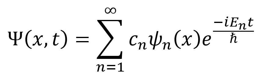
Physically, |cn|2 represents the probability that a measurement of the system’s energy would return a value of En. As such, an infinite sum of all the |cn|2 values is equal to 1. In addition, note that each Ψn(x,t) = ψn(x)e–iEnt/ℏ is known as a stationary state. The reason these solutions are called stationary states is because the expectation values of measurable quantities are independent of time when the system is in a stationary state (as a result of the time-dependent term canceling out).
Using wave functions
Once a wave function is known, it can be used to learn about the given quantum mechanical system. Though wave functions specify the state of a quantum mechanical system, this state usually cannot undergo measurement without altering the system, so the wave function must be interpreted probabilistically. The way the probabilistic interpretation is achieved will be explained over the course of this section.
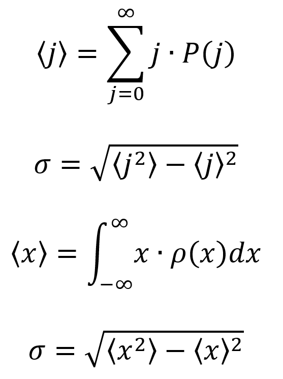
Before going further, it will be useful to understand some methods from probability. First, the expectation value is the average of all the possible outcomes of a measurement as weighted by their likelihood (it is not the most likely outcome as the name might suggest). Next, the standard deviation σ describes the spread of a distribution about an average value. Note that the square of the standard deviation is called the variance.
Equations for the expectation value and standard deviation are given as follows. The first equation computes the expectation value for a discrete variable j. Here, P(j) is the probability of measurement f(j) for a given j. The second equation is a convenient way to compute the standard deviation σ associated with the expectation value for j. The third equation computes the expectation value for a continuous function f(x). Here, ρ(x) is the probability density of x. When ρ(x) is integrated over an interval a to b, it gives the probability that measurement x will be found over that interval. The fourth equation the same as the second equation, but finds the standard deviation σ for the continuous variable x.
In quantum mechanics, operators are employed in place of measurable quantities such as position, momentum, and energy. These operators play a special role in the probabilistic interpretation of wave functions since they help one to compute an expectation value for the corresponding measurable quantity.
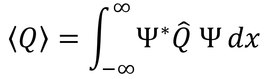
To compute the expectation value for a measurable quantity Q in quantum mechanics, the following equation is used. Here, Ψ is the time-dependent wave function, Ψ* is the complex conjugate of the time-dependent wave function, and Q̂ is the operator corresponding to Q.
Any quantum operator which corresponds to a classical dynamical variable can be expressed in terms of the momentum operator –iℏ(∂/∂x). By rewriting a given classical expression in terms of momentum p and then replacing every p within the expression by –iℏ(∂/∂x), the corresponding quantum operator is obtained. Below, a table of common quantum mechanical operators in 1D and 3D is given.

Heisenberg uncertainty principle
The Heisenberg uncertainty principle explains why quantum mechanics requires a probabilistic interpretation. According to the Heisenberg uncertainty principle, the more precisely the position of a particle is determined via some measurement, the less precisely its momentum can be known (and vice versa). The Heisenberg uncertainty principle is quantified by the following equation.
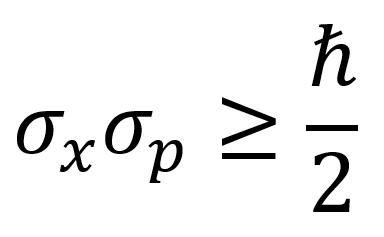
The reason for the Heisenberg uncertainty principle comes from the wave nature of matter (and not from the observer effect). For a sinusoidal wave, the wave itself is not really located at any particular site, it is instead spread out across the cycles of the sinusoid. For a pulse wave, the wave can be localized to the site of the pulse, but it does not really have a wavelength. There are also intermediate cases where the wavelength is somewhat poorly defined and the location is somewhat well-defined or vice-versa. Since the wavelength of a particle is related to the momentum by the de Broglie formula p = h/λ = 2πℏ/λ, this means that the interplay between the wavelength and the position applies to momentum and position as well. The Heisenberg uncertainty principle quantifies this interplay.
Some simple quantum mechanical systems
Infinite square well
The infinite square well is a system for which a particle’s V(x) = 0 when 0 ≤ x ≤ a and its V(x) = ∞ otherwise. Because the potential energy is infinite outside of the well, the probability of finding the particle there is zero. Inside the well, the time-independent Schrödinger equation is given as follows. This equation is the same as the classical simple harmonic oscillator.
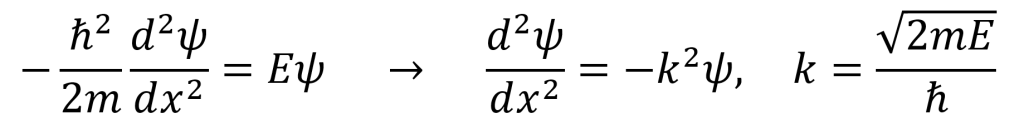
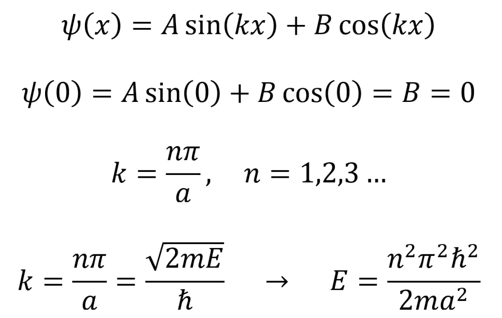
For the infinite square well, certain boundary conditions apply. In order for the wave function to be continuous, the wave function must equal zero once it reaches the walls, so ψ(0) = ψ(a) = 0. The general solution to the infinite square well differential equation is given as the first equation below. The boundary condition ψ(0) = 0 is employed in the second equation below. Since the coefficient B = 0, there are only sine solutions to the equation. Furthermore, if ψ(a) = 0, then Asin(ka) = 0. This means that k = nπ/a (where n = 1, 2, 3…) as given by the third equation below. The fourth equation below shows that this set of values for k leads to a set of possible discrete energy levels for the system
To find the constant A, the wave function ψ = Asin(nπx/a) must undergo normalization. As mentioned earlier, normalization is achieved by setting the normalization integral equal to 1 and solving for the constant A. Note that the time-independent Schrödinger equation can be utilized in the normalization integral since the exponential component of the time-dependent Schrödinger equation would cancel anyways.

Using this information, the wave functions for the infinite square well particle system are obtained. The time-independent and time-dependent wave functions are both displayed below at left and right respectively.

This infinite set of wave functions has some important properties. They possess discrete energies that increase by a factor of n2 with each level (and n = 1 is the ground state). The wave functions are also orthonormal. This property is described by the following equation. Here, δmn is the Kronecker delta and is defined below.

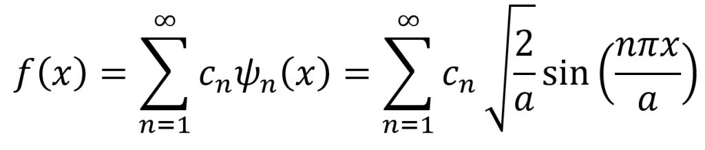
Another important property of these wave functions is completeness. This means that any function can be expressed as a linear combination of the time-independent wave functions ψn. The reason for this remarkable property is that the general solution (see below) is equivalent to a Fourier series.
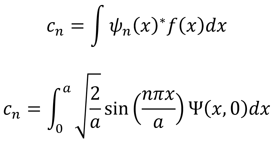
The first equation below can be employed to compute the nth coefficient cn. Here, f(x) = Ψ(x,0) which is an initial wave function. Note that the initial wave function can be any function Ψ(x,0) and the result will generate coefficients for that starting point. This first equation is derived using the orthonormality of the solution set. Note that the formula applies to most quantum mechanical systems since the properties of orthonormality and completeness hold for most quantum mechanical systems (though there are some exceptions). The second equation below computes the cn coefficients specifically for the infinite square well system.
Quantum harmonic oscillator
For the quantum harmonic oscillator, the potential energy in the Schrödinger equation is given by V(x) = 0.5kx2 = 0.5mω2x2. This means that the following time-independent Schrödinger equation needs to be solved.

There are two main methods for solving this differential equation. These include a ladder operator approach and a power series approach. Both of these methods are quite complicated and will not be covered here. The solutions for n = 0, 1, 2, 3, 4, 5 are given below. Here, Hn(y) is the nth Hermite polynomial. The first five Hermite polynomials and the corresponding energies for the system are given in the table. Note that the discrete energy levels for the quantum harmonic oscillator follow the form (n + 0.5)ћω.

As with any quantum mechanical system, the quantum harmonic oscillator is further described by the general time-dependent solution. To identify the coefficients cn for this general solution, Fourier’s trick is employed (see previous section) where f(x) is once again any initial wave function Ψ(x,0).
Quantum free particle
Though the classical free particle is a simple problem, there are some nuances which arise in the case of the quantum mechanical free particle which greatly complicate the system.
To start, the Schrödinger equation for the quantum free particle is given in the first equation below. Here, k = (2mE)0.5/ћ. Note that V(x) = 0 since there is no external potential acting on the particle. The second equation below is a general time-independent solution to the system in exponential form. The third equation below is the time-dependent solution to the system where the terms are multiplied by e–iEt/ћ. Realize that this general solution can be written as a single term by redefining k as ±(2mE)0.5/ћ. When k > 0, the solution is a wave propagating to the right. When k < 0, the solution is a wave propagating to the left.

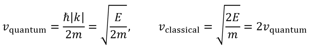
The speed of these propagating waves can be found by dividing the coefficient of t (which is ћk2/2m) by the coefficient of x (which is k). Since this is speed, the direction of the wave does not matter, so one can take the absolute value of k. By contrast, the speed of a classical particle is found by solving E = 0.5mv2, which gives a puzzling result that is twice as fast as the quantum particle.
Another challenge associated with the quantum free particle is that its wave function is non-normalizable (as shown below). Because of this, one can conclude that free particles cannot exist in stationary states. Equivalently, free particles never exhibit definite energies.

To resolve these issues with the quantum free particle, it has been found that the wave function of a quantum free particle actually carries a range of energies and speeds known as a wave packet. The solution for this wave packet involves the integral given by the first equation below and a function ϕ(k) given by the second equation below. This second equation allows one to determine ϕ(k) to fit a desired initial wave function Ψ(x,0). It was obtained using a mathematical tool called Plancherel’s theorem.

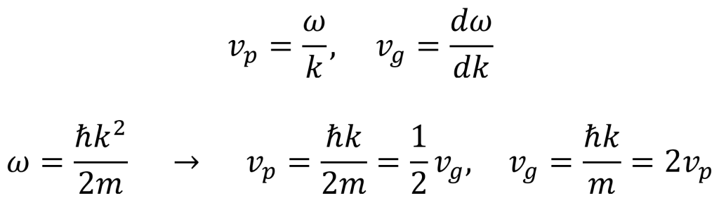
The above solution to the quantum free particle is now normalizable. Furthermore, the issue with the speed of the quantum free particle having a value twice as large as the speed of the classical free particle is fixed by considering a phenomenon known as group velocity. The waveform of the particle is an oscillating sinusoid (see image). This waveform includes an envelope, which represents the overall shape of the oscillations rather than the individual ripples. The group velocity vg is the speed of this envelope while the phase velocity vp is the speed of the ripples. It can be shown using the definitions of phase velocity and group velocity (see below) that the group velocity is twice the phase velocity, resolving the problem with the particle speed. The group velocity of the envelope is thus what actually corresponds to the speed of the particle.

Interlude on bound states and scattering states
To review, the solutions to the Schrödinger equation for the infinite square well and quantum harmonic oscillator were normalizable and labeled by a discrete index n while the solution to the Schrödinger equation for the free particle was not normalizable and was labeled by a continuous variable k.
The solutions which are normalizable and labeled by a discrete index are known as bound states. The solutions which are not normalizable and are labeled by a continuous variable are known scattering states.
Bound states and scattering states are related to certain classical mechanical phenomena. Bound states correspond to a classical particle in a potential well where the energy is not large enough for the particle to escape the well. Scattering states correspond to a particle which might be influenced by a potential but has a large enough energy to pass through the potential without getting trapped.
In quantum mechanics, bound states occur when E < V(∞) and E < V(–∞) since the phenomenon of quantum tunneling allows quantum particles to leak through any finite potential barrier. Scattering states occur when E > V(∞) or E > V(–∞). Since most potentials go to zero at infinity or negative infinity, this simplifies to bound states happening when E < 0 and scattering states happening when E > 0.
The infinite square well and the quantum harmonic oscillator represent bound states since V(x) goes to ∞ when x → ±∞. By contrast, the quantum free particle represents a scattering state since V(x) = 0 everywhere. However, there are also potentials which can result in both bound and scattering states. These kinds of potentials will be explored in the following sections.
Delta-function well
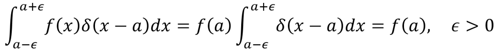
Recall that the Dirac delta function δ(x) is an infinitely high and infinitely narrow spike at the origin with an area equal to 1 (the area is obtained by integrating). The spike appears at the point a along the x axis when δ(x – a) is used. One important property of the Dirac delta function is that f(x)δ(x – a) = f(a)δ(x – a). By integrating both sides of the equation of this property, one can obtain the following useful expression. Note that a ± ϵ is used as the bounds since any positive value ϵ will then allow the bounds to encompass the Dirac delta function spike.
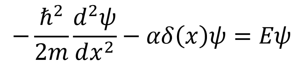
The delta-function well is a potential of the form –αδ(x) where α is a positive constant. As a result, the time-independent Schrödinger equation for the delta-function well system is given as follows. This equation has solutions that yield bound states when E < 0 and scattering states when E > 0.
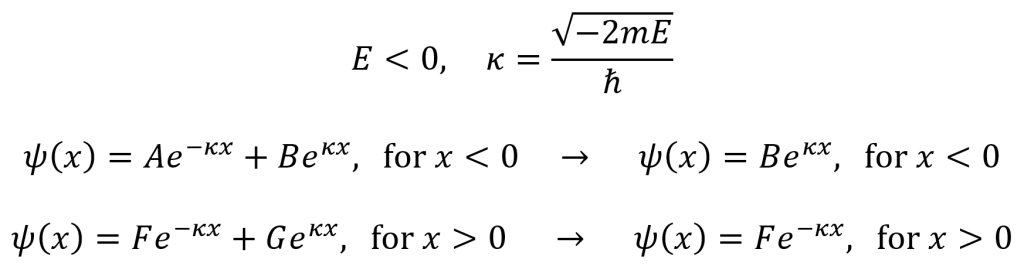
For the bound states where E < 0, the general solutions are given by equations below. The substitution κ is defined by the first equation below, the second equation below is the general solution for x < 0, and the third equation below is the general solution for x > 0. (Since E is assumed to have a negative value, κ is real and positive). Note that V(x) = 0 for x < 0 and x > 0. In the solution for x < 0, the Ae–κx term explodes as x → –∞, so A must equal zero. In the solution for x > 0, the Feκx term explodes as x → ∞, so F must equal zero.
To combine these equations, one must use appropriate boundary conditions at x = 0. For any quantum system, ψ is continuous and dψ/dt is continuous except at points where the potential is infinite. The requirement for ψ to exhibit continuity means that F = B at x = 0. As a result, the solution for the bound states can be concisely stated as follows. In addition, a plot of the delta-function well’s bound state time-independent wave function is given below.


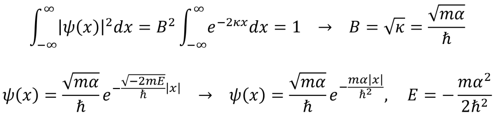
The presence of the delta function influences the energy E. To find the energy, one can integrate the time-independent Schrödinger equation for the delta-function well system. By making the bounds of integration ±ϵ and then taking the limit as ϵ approaches zero, the integral works only on the negative spike of the delta function at x = 0. The result for the energy is at the end of the following set of equations.

As seen above, the delta-function well only exhibits a single bound state energy E. By normalizing the wave function ψ(x) = Be–κ|x|, the constant B is found (as seen in the first equation below). The second equation below describes the single bound state wave function and reiterates the single bound state energy associated with this wave function.
For the scattering states where E > 0, the general solutions are given by equations below. The substitution k is defined by the first equation below, the second equation below is the general solution for x < 0, and the third equation below is the general solution for x > 0. (Since E is assumed to have a positive value, k is real and positive). Note that V(x) = 0 for x < 0 and x > 0. None of the terms explode this time, so none of the terms can be ruled out as equal to zero.

As a consequence of the requirement for ψ(x) to be continuous at x = 0, the following equation involving the constants A, B, F, and G must hold true. This is the first boundary condition.

There is also a second boundary condition which involves dψ/dx. Recall the following step (see first equation below) from the process of integrating the Schrödinger equation. To implement this step, the derivatives of ψ(x) (see second equation below) are found and then the limits of these derivatives from the left and right directions are taken (see third equation below). Since ψ(0) = A + B as seen in the equation above, the second boundary condition can be given as the final equation below.

By rearranging the final equation above and substituting in a parameter β = mα/ћ2k, the following expression is obtained. This expression is a compact way of writing the second boundary condition.

These two boundary conditions provide two equations, but there are four unknowns in these equations (five unknowns if k is included). Despite this, the physical significance of the unknown constants can be helpful. When eikx is multiplied by the factor for time-dependence e–iEt/ћ, it gives rise to a wave propagating to the right. When e–ikx is multiplied by the factor for time-dependence e–iEt/ћ, it gives rise to a wave propagating to the left. As a result, the constants describe the amplitudes of various waves. A is the amplitude of a wave moving to the right on the x < 0 side of the delta-function potential, B is the amplitude of a wave moving to the left on the x < 0 side of the delta-function potential, F is the amplitude of a wave moving to the right on the x > 0 side of the delta-function potential, and G is the amplitude of a wave moving to the left on the x > 0 side of the delta-function potential.
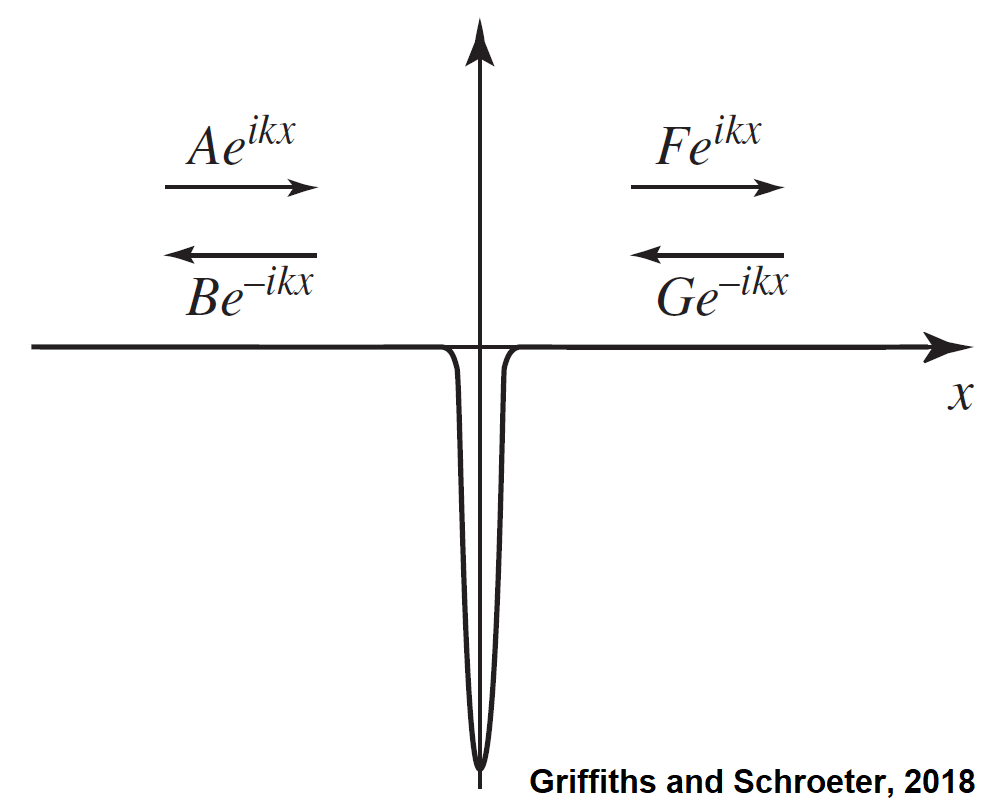
In a typical experiment on this type of system, particles are fired from one side of the delta-function potential, the left or the right. If the particles are coming from the left (moving to the right), the term with G will equal zero. If the particles are coming from the right (moving to the left), the term with A will equal zero. This can be understood intuitively by examining the figure above.
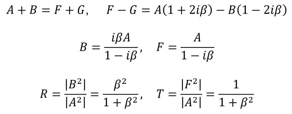
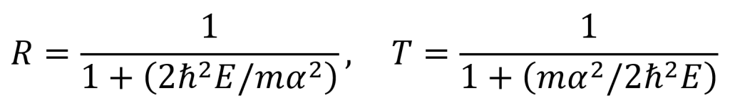
As an example, for the case of particles fired from the left (moving to the right), A is the amplitude of the incident wave, B is the amplitude of the reflected wave, and F is the amplitude of the transmitted wave. The equations of the two boundary conditions are reiterated in the first line below. By solving these equations, the second line of expressions is found. Since the probability of finding a particle at a certain location is |Ψ|2, the relative probability R of an incident particle undergoing reflection and the relative probability T of an incident particle undergoing transmission are given by the third line of expressions below.
Also for the example case of particles fired from the left (moving to the right), by substituting back from β = mα/ћ2k and k = (2mE)0.5/ћ to get the expressions in terms of energy, the following equations are obtained for the reflection and transmission relative probabilities.
By performing the same process, but with A = 0 instead of G = 0, corresponding equations can be found for the case of particles fired from the right (moving towards the left).
It is important to note that, since these scattering wave functions are not normalizable, they do not actually represent possible particle states. To solve this problem, one must construct normalizable linear combinations of the stationary states in a manner similar to that performed with the quantum free particle system. In this way, wave packets will occur and the actual particles will be described by the range of energies of the wave packets. Because the actual normalizable system exhibits a range of energies, the probabilities R and T should be thought of as approximate measures of reflection and transmission for particles with energies in the vicinity of E.
Finite square well
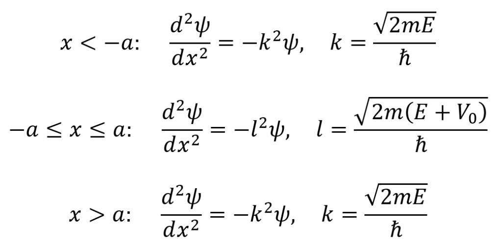
The finite square well is a system for which a particle’s V(x) = –V0 when –a ≤ x ≤ a and its V(x) = 0 otherwise. For this system, the Schrödinger equation is given as follows for the conditions x < –a, –a ≤ x ≤ a, and x > a. Note that the equations for x < –a and x > a are the same since V(x) = 0 in both cases (but the boundary conditions will differ as will be explained soon). As with the Delta-function potential well, the finite square well has both bound states (with E < 0) and scattering states (with E > 0). First, the bound states with E < 0 will be considered. In this case, the Schrödinger equations for the finite square well are as follows.


For the cases of x < –a and x > a where V(x) = 0, the general solutions to the Schrödinger equation are respectively Ae–κx + Beκx and Fe–κx + Geκx where A, B, F, and G are arbitrary constants. In the x < –a case, the Ae–κx term blows up as x → –∞, making this term physically invalid. As a result, the physically admissible solution is ψ(x) = Beκx. In the x > a case, the Geκx term blows up as as x → ∞, making this term physically invalid. As a result, the physically admissible solution is ψ(x) = Fe–κx. For the case of –a ≤ x ≤ a, the general solution to the Schrödinger equation is ψ(x) = Csin(lx) + Dcos(lx). Note that, because E must be greater than the minimum potential energy Vmin = –V0, the value of l ends up real and positive (even though E is also negative). These solutions are summarized by the following equations.

Since the potential V(x) = –V0 is an even function (symmetric about the y axis), one can choose to write the solutions to the wave function as either even or odd. This comes from some properties of the time-independent Schrödinger equation. Next, it is again important to constrain these solutions using the boundary conditions which require the continuity of ψ(x) and dψ/dx at ±a.
For the even solutions, the constant C in ψ(x) = Csin(lx) + Dcos(lx) is zero. Because C = 0, the remaining equation is the even function ψ(x) = Dcos(lx) for –a ≤ x ≤ a. So, the continuity of ψ(x) and dψ/dx at +a necessitates the following two equations to hold true. The third equation comes from dividing the second equation by the first equation to solve for κ.

For the odd solutions, the constant D in ψ(x) = Csin(lx) + Dcos(lx) is zero. Because D = 0, the remaining equation is the odd function ψ(x) = Dsin(lx) for –a ≤ x ≤ a. So, the continuity of ψ(x) and dψ/dx at +a necessitates the following two equations to hold true. The third equation comes from dividing the second equation by the first equation to solve for κ.

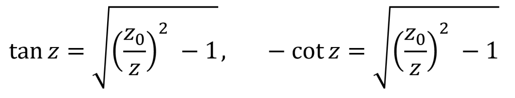
As κ and l are both functions of E, the κ = ltan(la) and κ = –lcot(la) equations can be solved for E. To do this, it is convenient to use the notation z = la and z0 = (a/ћ)(2mV0)0.5. Simplifying the κ = ltan(la) and κ = –lcot(la) equations using this notation gives the following results. These equations can be solved numerically for z or graphically for z by looking for points of intersection (after obtaining z, E is easily computed).
Let us consider the tan(z) equation. There are two limiting cases of interest. These include a well which is wide and deep and a well which is shallow and narrow. Though not included in these notes, similar calculations can be performed for the –cot(z) equation.
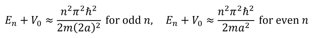
For a wide and deep well, the value of z0 is large. Intersections between the curves of tan(zn) and ((z0/zn)2 – 1)0.5 occur at nπ/2 for odd n and at nπ for even n. This leads to the following equations which describe values of En. From this outcome, it can be seen that infinite V0 results in the infinite square well case with an infinite number of bound states. However, for any finite square well, there are only a finite number of bound states.
For a shallow and narrow well, the value of z0 is small. As the value of z0 decreases, fewer and fewer bound states exist. Once z0 is smaller than π/2, there is only one bound state (which is an even bound state). Interestingly, no matter how small the well, this one bound state always persists.
The scattering states, which occur when E > 0, will now be considered. In this case, the Schrödinger equations for the finite square well are as follows.
The general solutions to the Schrödinger equation for the finite square well’s scattering states are as follows.

But recall that in a typical scattering experiment, particles are fired from one side of the delta-function potential, the left or the right. Here it will be assumed that the particles are fired from the left side of the well (moving towards the right). Note that similar calculations could be performed for the opposite case. With this assumption, one can realize that the coefficient A represents the incident (from the left) wave’s amplitude, the coefficient B represents the reflected wave’s amplitude, and the coefficient F represents the transmitted (to the right) wave’s amplitude. Finally, the coefficient G = 0 since there is not an incident wave from the right moving towards the left.
There are four boundary conditions, continuity of ψ(x) at ±a and continuity of dψ/dx at ±a. These boundary conditions yield the following equations.

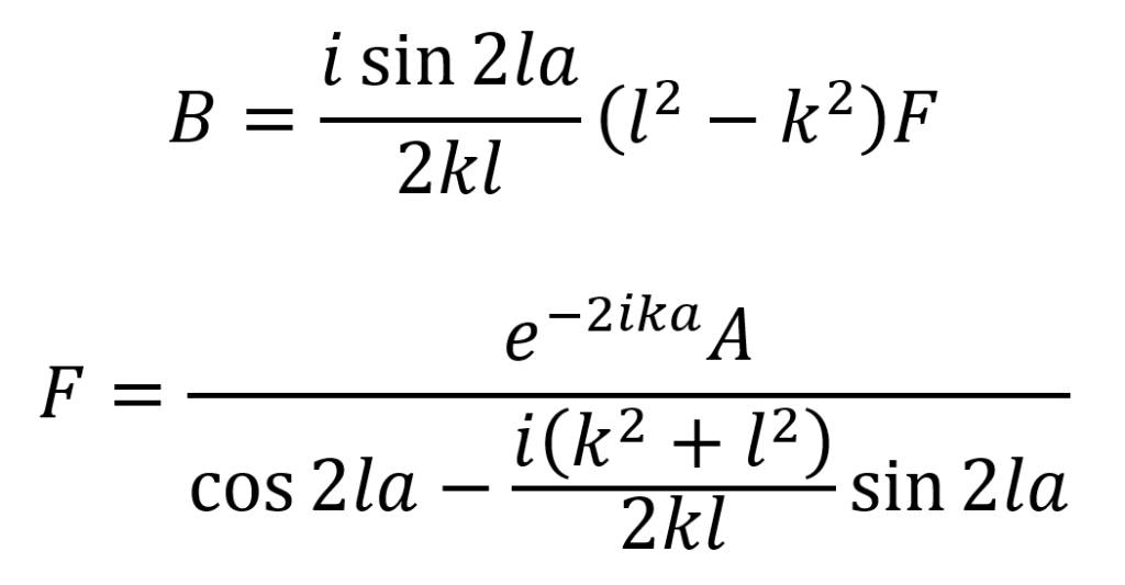
With the above equations, one can eliminate C and D and subsequently solve the system for B and F. This yields the equations below for B and F.
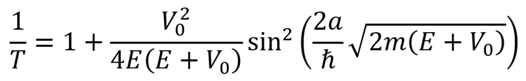
As with the delta-function well, a transmission coefficient T = |F|2/|A|2 can be computed across the finite square well. Recall that T represents the probability of the particle undergoing transmission across the well (in this case when moving from the right side to the left side). The probability of the particle undergoing reflection is R = 1 – T.

Since 1/T equals the equation below, whenever the sine squared term is zero, the probability of transmission T = 1.
Recall that a sine (or sine squared) term is zero when the function inside of it equals nπ such that n is any integer.

Remarkably, the above equation is the same as the one which describes the infinite square well’s energies. But realize that, for the finite square well, this only holds in the case of T = 1.
Reference: Griffiths, D. J., & Schroeter, D. F. (2018). Introduction to Quantum Mechanics (3rd ed.). Cambridge University Press. https://doi.org/DOI: 10.1017/9781316995433
Cover image source: wikimedia.org
