Author: logancollins

     Most ideologies include methods for finding reasons to live. But after seeing historical tragedies in which such methods have led to tremendous suffering, some have given up on the idea of purpose. This is not an entirely unreasonable response, but I would argue that it still represents an unjustifiably pessimistic outlook. Although most systems of existential meaning suffer from crippling flaws, such flaws do not invalidate the possibility of purpose. Religious, political, and philosophical approaches have been applied towards resolving the question of existential purpose (Triandis, 2008). Each system possesses certain merits, but they are incomplete since their theoretical frameworks lacks rigor and data. In this essay, I will discuss a toolset and a general philosophical framework which may aid efforts to construct a meaningful world. I propose that existential meaning arises from specific computational structures encoded in matter which can be understood and engineered using the empirical and self-correcting process of scientific inquiry.

     Religious thinkers suggest that specific dogma associated with a given belief system provide meaning. They argue that the purpose of life involves fulfilling certain natural laws which they associate with deities, scriptures, and prophets. However, religious ideologies lack strong empirical support for their dogmas. This may arise from religious doctrines not including effective ways for them to evolve as new knowledge is acquired and circumstances change (Emerson & Hartman, 2006). It should be noted that some religions possess a greater level of flexibility than others. For instance, followers of Hinduism have demonstrated openness to their religion evolving as scientific knowledge provides new insights about the universe. Varadaraja Raman has written on deconstructing the schism between Hindu spirituality and science by reinterpreting Hindu ideas as metaphors for scientific concepts (Raman, 2009). In addition, some followers of the Vedanta philosophy subscribe to a nondualist view of the universe and have made attempts to reconcile Hindu beliefs with new scientific findings (Dorman, 2011). However, other Hindu philosophies have remained bound to tradition, rejected concepts like evolution by natural selection, and even embraced radical postmodernist characterizations of rationality as a tool for oppression (Raman, 2012). Since many religions have exhibited staticity in their interpretations of purpose when new data contradicts their dogma, I propose that existing and past religions have created approximate models for purpose, but fallen short of their ultimate goals.

     Political strategies for finding meaning often involve creating identity via tribal association with certain values while rejecting outgroups which deviate from said values. According to a meta-analysis performed by Jost et al., both conservatives and liberals possess existential motivations driven by specific fears associated with opposing values (Jost, Stern, Rule, & Sterling, 2017). For conservatives, the data indicated fear of governmental control, racial minorities, and social changes that conflict with traditional views. Among liberals, the data indicated that threatening circumstances trigger an increase in tendencies towards strong moralization of political issues. Across political affiliations, such tribalistic behaviors may correlate with the same psychologies which drive religious and philosophical approaches to uncovering existential meaning (Norris & Inglehart, 2011). This is not inherently wrong, but it does reframe politics as holding similarities to religion in that politics may only provide approximations in its pursuit of meaning. Furthermore, political techniques have so far failed to create stable utopian societies, though secular political systems have debatably realized improvements over theocratic systems (Lilla, 2008).

     Stoic philosophers such as Albert Camus argue that accepting absurdity may represent a superior way of living (Camus, 2013). Stoicism seeks to ignore value and so avoid existential dread (Nagel, 1971). But stoicism is paradoxical in that it denies the phenomenological existence of value (Block, 1995; D. J. Chalmers, 1995; Nagel, 1974). Stoics may claim to live passively, but they will always fail to exercise consistency in this doctrine since value is a fundamental constituent of reality. Any entity will possess at least some degree of motivation, regardless of whether the entity wants to possess said motivations. The universal existence of motivation can be illustrated by causality in natural systems. For this argument, I take the nondualist position that consciousness is identical to specific physical processes and does not possess a supernatural component. Consider a rock which rolls down a hill and strikes a second rock. In this scenario, the second rock cannot prevent itself from having a reaction. Biological organisms are no exception to causality. From atoms to galaxies, the cosmos is driven by change. As much as a stoic may try to condition him or herself against reaction, physical reality remains intrinsically causal, so this task will ultimately be in vain.

     To provide a contextual background for my proposal that existential meaning is encoded in matter, I will introduce a physical argument for panpsychism. Despite its past association with metaphysics, panpsychism is rekindling among contemporary thinkers as an explanation for consciousness (Strawson, 2006). Integrated information theory or IIT (Oizumi, Albantakis, & Tononi, 2014) is a mathematical formulation which seeks to quantify consciousness using the information arising from dynamical systems. Galen Strawson has argued that IIT implies panpsychism since all physical structures contain some amount of information (Strawson, 2006). Furthermore, Adam Barrett has proposed modifications to IIT which may help account for fundamental physical interpretations of the universe like quantum field theory (Barrett, 2014). Panpsychic descriptions of reality are reentering philosophical and scientific discourse as new data are acquired and new theoretical interpretations develop.

     But many still view the idea that inanimate objects may possess primitive qualia as ludicrous. To counter this presumption, consider a fragment of quartz resting on a ridge. As the sun rises, photons excite the atoms on the crystal’s surface, causing thermal oscillations to propagate into the quartz. This thermal diffusion is modulated by crystallographic defects, causing a heterogeneous distribution of heat inside the rock. As dusk falls, the quartz fragment begins to cool, emitting heat at varying rates across the surface. The particular rates are influenced directly by this quartz specimen’s pattern of internal defects. Next, consider a mouse, also located on the ridge. As the sun rises, photons excite the retinaldehyde molecules in the mouse’s eyes, triggering signal transduction via electrochemical systems. This signal moves into the mouse’s brain, where it propagates through a series of neural pathways, causing a heterogeneous distribution of neural activity. Soon, the signal’s interaction with preexisting brain structures is translated into a motor action; the mouse blinks and looks away from the bright illumination. The particular motor response is modulated by the structural organization of this mouse’s brain at the given time. The quartz and the mouse both receive sensory inputs, process them according to internal properties, and then give motor outputs. Although the rock’s “brain” is much more disorganized and chaotic than the mouse’s brain, it operates by the same basic principles and could plausibly experience a primitive form of consciousness. As such, the possibility of panpsychism cannot be readily dismissed as absurd or metaphysical.

     Another prominent objection to panpsychism arises from brain processes which occur in a subconscious fashion. For instance, activity in the primary visual cortex (V1) does not correlate with conscious visual experience except for a few special cases (Crick & Koch, 1995) (Boyer, Harrison, & Ro, 2005) (Boehler, Schoenfeld, Heinze, & Hopf, 2008). However, the presence of subconscious neural events does not necessarily indicate that the said events are subconscious from the viewpoint of their associated anatomies. Instead, anatomical structures like V1 may experience their own independent qualia. The full informational content of their perceptions may not be transmitted or translated into the brain areas like the prefrontal cortex (PFC) which can be identified with a patient’s sense of self (Mitchell, Banaji, & Macrae, 2005). Of course, some data does transfer into higher brain regions to facilitate processes like vision, but the information undergoes an extensive series of transformations before arriving at the PFC and other regions associated with conscious processing. For this reason, the “unconscious anatomies” objection is insufficient to invalidate panpsychism.

     Under the assumption of panpsychism or the similar description provided by protopanpsychism (Chalmers, 2015), cognitive states are identical to configurations of matter and energy. As emotions like joy, anger, wonder, sadness, and love emerge from functional circuits in the brain, the same emotions may emerge from informationally equivalent circuits in other substrates like classical computers equipped with biologically-realistic software models or neuromorphic semiconductor devices (Koene, 2013). This reasoning applies to feelings of existential meaning as well. If the emotions associated with fulfillment and purpose are encoded in physical matter, then they represent an intrinsic property of the universe. As such, the possibility of existential meaning cannot be dismissed on the grounds that it arises as an irrational psychological construction, though psychological biases still must be taken into consideration.

     Feelings of existential meaning come in many flavors and magnitudes, some of which may represent objectively “better” states than others. To explain this principle, I will describe several illustrative fictional scenarios. First, consider a venture capitalist named Aiko, a man who enjoys the thrill of financial competition. Aiko feels some level of fulfillment from his pursuits. Despite this, Aiko also experiences loneliness since he has not maintained close relationships with his family. Now consider Anastasia, a feminist intellectual who has made notable strides towards gender equality. By comparison to Aiko, Anastasia experiences a stronger sense of fulfillment from her work as well as lesser misgivings from the sacrifices she has made in other areas. In a somewhat fanciful exploration, consider an unbiased spirit which decides to inhabit Aiko’s mind and then Anastasia’s mind. This spirit is assumed to exhibit perfect rationality. Upon comparing the two people’s internal states, the spirit concludes that it would prefer Anastasia’s emotional experiences over Aiko’s emotional experiences. This account demonstrates the idea that purpose can manifest differently across individuals, that such differences can undergo objective comparison, and that some states may represent objectively superior qualia.

     Despite this, I would argue that the events which trigger emotional states associated with purpose are irrelevant to existential meaning. Distinct sets of events can still cause distinct emotional states, but only the resulting emotions themselves define purpose. To understand this, consider a factory worker called Akhmed, who was born with a mutation which influenced his neural development such that he easily gains feelings of fulfillment even in mundane situations. Also consider an influential political leader named Carlos, who was born with an unfortunate susceptibility to clinical depression. Akhmed’s feeling of purpose in his monotonous factory work represents an objectively better state than Carlos’s sensation of meaninglessness even as Carlos facilitates widespread social improvements. Note that this scenario focuses upon the emotional states of the specific physical subsystems corresponding to Akhmed and Carlos, not on the physical subsystems corresponding to the people who Carlos has helped. The qualia involved in an emotion, rather than the causes for said qualia, are necessary for explaining the emotion’s value. Although meaning can vary across individuals, informatic circuits which underlie meaning may provide a route for quantifying purpose’s value and for pursuing existential fulfillment with greater methodological precision.

     From a practical perspective, this proposal indicates that deliberate creation of positive emotional states associated with purpose is an intrinsically worthwhile pursuit, but also that this pursuit must undergo consideration in a larger context. I suggest that it may not always be ethical for a subsystem of the universe such as an individual human to create positive emotional states within herself if the process causes harm to others. Note that a full exploration of potential physical bases for morality is beyond the scope of this essay. But despite the conflicts raised by altering emotional states in a heterogeneously distributed manner, reconfiguring matter on larger scales towards positive emotional states represents a clearer imperative.

     In some ways, earlier approaches to the question of existential purpose have already suggested the goal of reconfiguring matter towards meaningful emotional states. But certain religious, political, and philosophical approaches have demonstrated more success than others. In cases like Islamic fundamentalism, Christofascism (Sölle, 1970), Nazism, and social Darwinism, their attempts have backfired and caused widespread harm rather than improvement. But as mentioned, such approaches have suffered from poor theoretical and empirical rigor in their development. I would argue that using evidence-based methods towards creating a better tomorrow will facilitate the creation of policies, technologies, and ethical guidelines which possess sufficient theoretical and empirical rigor to simultaneously maximize the likelihood of widespread beneficial results and minimize the likelihood of widespread harmful results. Existential meaning is tied to physical reality and so can be engineered. In order to create existential meaning without falling prey to the same mistakes observed through history, we must utilize empirical methods to guide the construction of a bright future in which positive emotions are recognized as physical expressions of purpose and effective strategies for maintaining such emotions are implemented.

References

Barrett, A. (2014). An integration of integrated information theory with fundamental physics. Frontiers in Psychology. Retrieved from https://www.frontiersin.org/article/10.3389/fpsyg.2014.00063

Block, N. (1995). On a confusion about a function of consciousness. Behavioral and Brain Sciences, 18(2), 227–247.

Boehler, C. N., Schoenfeld, M. A., Heinze, H.-J., & Hopf, J.-M. (2008). Rapid recurrent processing gates awareness in primary visual cortex. Proceedings of the National Academy of Sciences, 105(25), 8742 LP-8747. Retrieved from http://www.pnas.org/content/105/25/8742.abstract

Boyer, J. L., Harrison, S., & Ro, T. (2005). Unconscious processing of orientation and color without primary visual cortex. Proceedings of the National Academy of Sciences of the United States of America, 102(46), 16875 LP-16879. Retrieved from http://www.pnas.org/content/102/46/16875.abstract

Camus, A. (2013). The myth of Sisyphus. Penguin UK.

Chalmers, D. (2015). Panpsychism and panprotopsychism. Consciousness in the Physical World: Perspectives on Russellian Monism, 246.

Chalmers, D. J. (1995). Facing up to the problem of consciousness. Journal of Consciousness Studies, 2(3), 200–219.

Crick, F., & Koch, C. (1995). Are we aware of neural activity in primary visual cortex? Nature, 375(6527), 121–123.

Dorman, E. (2011). Hinduism and Science: The State of the South Asian Science and Religion Discourse. Zygon®, 46(3), 593–619. http://doi.org/10.1111/j.1467-9744.2011.01201.x

Emerson, M. O., & Hartman, D. (2006). The Rise of Religious Fundamentalism. Annual Review of Sociology, 32(1), 127–144. http://doi.org/10.1146/annurev.soc.32.061604.123141

Jost, J. T., Stern, C., Rule, N. O., & Sterling, J. (2017). The Politics of Fear: Is There an Ideological Asymmetry in Existential Motivation? Social Cognition, 35(4), 324–353. http://doi.org/10.1521/soco.2017.35.4.324

Koene, R. A. (2013). Uploading to Substrate‐Independent Minds. The Transhumanist Reader: Classical and Contemporary Essays on the Science, Technology, and Philosophy of the Human Future, 146–156.

Lilla, M. (2008). The Stillborn God: Religion, Politics, and the Modern West. Vintage Books. Retrieved from https://books.google.com/books?id=nfSMDQAAQBAJ

Mitchell, J. P., Banaji, M. R., & Macrae, C. N. (2005). The Link between Social Cognition and Self-referential Thought in the Medial Prefrontal Cortex. Journal of Cognitive Neuroscience, 17(8), 1306–1315. http://doi.org/10.1162/0898929055002418

Nagel, T. (1971). The absurd. The Journal of Philosophy, 68(20), 716–727.

Nagel, T. (1974). What Is It Like to Be a Bat? The Philosophical Review, 83(4), 435–450. http://doi.org/10.2307/2183914

Norris, P., & Inglehart, R. (2011). Sacred and Secular: Religion and Politics Worldwide. Cambridge University Press. Retrieved from https://books.google.com/books?id=ObwtZ36m1hwC

Oizumi, M., Albantakis, L., & Tononi, G. (2014). From the Phenomenology to the Mechanisms of Consciousness: Integrated Information Theory 3.0. PLOS Computational Biology, 10(5), e1003588. Retrieved from https://doi.org/10.1371/journal.pcbi.1003588

Raman, V. (2009). Truth and Tension in Science and Religion. Beech River Books. Retrieved from https://books.google.com/books?id=UggdrSiVvhsC

Raman, V. (2012). Hinduism and Science: Some Reflections. Zygon®, 47(3), 549–574. http://doi.org/10.1111/j.1467-9744.2012.01274.x

Sölle, D. (1970). Beyond Mere Obedience: Reflections on a Christian Ethic for the Future. Augsburg Publishing House. Retrieved from https://books.google.com/books?id=zbeCGwAACAAJ

Strawson, G. (2006). Realistic monism: why physicalism entails panpsychism.

Triandis, H. C. (2008). Fooling Ourselves: Self-Deception in Politics, Religion, and Terrorism: Self-Deception in Politics, Religion, and Terrorism. ABC-CLIO. Retrieved from https://books.google.com/books?id=GGdrumE1JuYC

 

PDF Version: Notes on Upconversion Nanoparticles – Logan Thrasher Collins

Background and Overview

• Photoluminescence spectroscopy (also called fluorescence spectroscopy) uses electromagnetic radiation to excite electrons in various materials. Photons are emitted from the materials as the electrons return to lower energy states. In biology and biomedicine, photoluminescence spectroscopy provides a noninvasive tool which allows for visualization of biological processes over a wide range of scales (subcellular to macroscale).
• Many biological applications of fluorescence spectroscopy require exogenous contrast agents like organic dyes, fluorescent proteins, quantum dots, and metal complexes. But such agents often possess limitations including (i) low signal-to-background ratio as a result of tissue autofluorescence and scattering when short wavelengths are used, (ii) low penetration depth when UV or visible light excitation is used as well as when UV or visible light are emitted, (iii) potential DNA damage from short wavelengths like UV, and (iv) potential toxicity of contrast agents containing heavy metals like cadmium and lead.
• Near-infrared (NIR) wavelengths provide a potentially superior alternative to other types of excitation for many situations. Biological tissue exhibits “optical transparency” in the NIR range of 700-1100 nm, allowing for deeper tissue penetration. In addition, NIR usually causes less autofluorescence and scattering. Some other alternatives exist, but these generally require expensive ultrashort pulsed lasers, so they are often less practical than NIR techniques.
• Lanthanide-doped upconversion nanoparticles (UCNPs) absorb two or more low-energy photons and emit a single photon with a higher energy. In this way, the long wavelengths of NIR can be converted to shorter wavelength radiation like visible light and UV upon emission.

Nanochemistry of UCNPs

• In lanthanide-doped UCNPs, trivalent lanthanide cations (elements with atomic numbers in the range of 57-71 which possess a +3 charge) are embedded in a chosen dielectric lattice that is 100 nm or less in diameter. Dielectric lattices are crystalline solids which possess a net polarity due to the contributions of individual atoms within the lattice. This polarization can be quantified by an optically-measureable lattice dielectric constant.
• Using appropriate lanthanide dopants allows for wavelength-selective upconversion. NIR excitation wavelengths are converted to specific emission wavelengths. For instance, NIR can be selectively converted to blue light by some UCNPs and to ultraviolet by other UCNPs.
• When UCNPs are excited by NIR light, electrons in the trivalent lanthanide cations undergo 4f-4f orbital electronic transitions. Since the 5s and 5p shells provide an electronic shielding effect, the transitions are sharp rather than broad. The 4f-4f transitions which occur in UCNPs would ordinarily be forbidden by quantum mechanical laws, but interactions of the lanthanide ions with the crystal lattice of the nanoparticle allow “orbital mixing” which facilitates such transitions.
• The upconversion photoluminescence intensity of UCNPs exhibits a nonlinear dependence of the number of excitation photons required to induce photoluminescence from the nanoparticles. Here, the number of excitation photons is given by n, K is a material-specific constant, and P is the power of the laser (called a pump laser) used to excite the nanoparticles. It should be noted that a saturation effect occurs at high excitation energy densities, leading to a decrease in the apparent value of n.

• Upconversion quantum yield (UCQY) is defined as the number of photons emitted per photon absorbed. It is proportional to the ratio of the emitted upconversion light intensity to the absorbed light intensity. Using these relations and the equation for upconversion photoluminescence intensity, the equation below can be derived. Here, α is an absorption constant that is specific to the material and the excitation wavelength.

Upconversion Mechanisms

• There are five basic upconversion mechanisms including excited-state absorption, energy transfer upconversion, cooperative sensitization upconversion, cross relaxation, and photon avalanche.
• Excited-state absorption: multiple photons are absorbed by a single lanthanide ion, exciting electrons up a ladder-like series of energy levels. It should be noted that only certain lanthanides possess the proper characteristics for this mechanism to occur (Ho³⁺, Er³⁺, Nd³⁺, and Tm³⁺) when commercially-available diode lasers are used (which usually have incident wavelengths of around 975 or 808 nm). The relevant energy levels are called G, E1, and E2 (for ground state, excited state 1, and excited state 2). Electrons in the E1 excited state have long lifetimes before they return to the ground state G. As such, after an electron is excited to E1, it remains there for long enough that it can be promoted to E2 by another photon. When the electron decays from E2 all the way to G, this large change in energy causes a photon with a shorter wavelength to be emitted (shorter than the photons involved in the excitation).
• Energy transfer upconversion: a lanthanide ion called the sensitizer absorbs a photon and is excited to E1, then transfers its energy to an ion called the activator. The sensitizer then decays back to G. This occurs twice, causing the activator to be excited to E1 and then to E2. When the electron decays from E2 all the way to G, this large change in energy again causes a photon with a shorter wavelength to be emitted. Some of the most efficient UCNPs used for biomedical purposes operate by energy transfer upconversion and involve sensitizer/activator ion pairs of Yb³⁺/Tm³⁺, Yb³⁺/Er³⁺, or Yb³⁺/Ho³⁺ with excitation wavelengths of about 975 nm. The Yb³⁺ ion does not have an E2 energy level, it can only be excited from G to E1. This makes the upconversion process more efficient since the two energy levels of Yb³⁺ cannot cause cross-relaxations (a phenomenon which has a deleterious effect on upconversion). In addition to Yb³⁺-based UCNPs that work by energy transfer upconverion, some single-lanthanide UCNPs have also been developed. In these, the single type of lanthanide ion acts as a sensitizer and an activator.
• Cooperative sensitization upconversion: two ions of the same type absorb excitation photons and are excited to E1 states. Next, both ions simultaneously transfer energy to a third ion (which can be of a different type) and excite the third ion to its own E1 state. In this case, the E1 state of the third ion is twice as energetic as the E1 states of the other two ions. When the third ion returns to its ground state, it releases a photon with a shorter wavelength than the incident photons. Cooperative sensitization upconversion is much less efficient than the other mechanisms, but it may have some advantages for high-resolution imaging applications. The cooperative sensitization mechanism has been reported to occur with Yb³⁺/Tb³⁺, Yb³⁺/Eu³⁺, and Yb³⁺/Pr³⁺ ion pairs.
• Cross relaxation: an ion is excited to E2 and then transfers its energy to a second ion as it returns to E1, exciting the second ion to E1. This mechanism depends on  ion-ion interactions, so it is closely associated with dopant ion concentration. It can cause quenching at high concentrations, but tuning ion concentrations allows modulation of emitted light colors via other mechanisms. Note that cross relaxation on its own does not cause upconversion, but that it can influence upconversion events as other steps occur.
• Photon avalanche: processes of excited-state absorption and cross-relaxation interact to create a positive feedback loop. Minimal upconversion occurs until a threshold of power input is passed, but the upconverted photoluminescence intensity vastly increases once the threshold has been exceeded. First, excited-state absorption causes an ion at E1 to transition into E2. Then this ion transfers its energy to a second ion, its electron goes down to E1, and the second ion’s electron is excited from G to E1 by cross relaxation. Last, the second ion transfers its energy to a third ion, resulting in two ions at the E1 state by the end of the loop. In this way, more and more ions are excited to the E1 state as the loop repeats (two, four, eight, etc.) Some of the ions in the E2 state (from the first step) will decay to G, causing upconverted photons to be released.

 

Reference: Chen, G., Qiu, H., Prasad, P. N., & Chen, X. (2014). Upconversion Nanoparticles: Design, Nanochemistry, and Applications in Theranostics. Chemical Reviews, 114(10), 5161–5214. http://doi.org/10.1021/cr400425h

PDF Version: Notes on Quantum Mechanics – Logan Thrasher Collins

Fundamentals

• The Rydberg equation gives the wavelength of the photon emitted when an electron moves from an excited state n_i to a lower energy level n_f. Here, R is the Rydberg constant, R = 1.09710⁷ m^-1.

• For electromagnetic waves the speed of light c, the frequency, and the wavelength are related by f=c/λ.
• Particles exhibit a wavelength called the de Broglie wavelength, which can be computed using Planck’s constant h = 6.62610^-34 m²kg/s over the momentum mv.

• The energy of a wave (in J) is given by the equation below.

The Schrӧdinger Equation

• Any particle can be described by a wave function ψ(x,y,z,t). In 1D, the wave function is ψ(x,t). The physical meaning of the wave function will be explained in the next section.
• The 1D Schrӧdinger equation relates a particle’s wave function ψ(x,t), its potential energy V, and its total energy. Solving this differential equation gives a formula for the wave function of a particle. The symbol ℏ represents the reduced Planck’s constant, h/2π.

• For the 3D case, the Laplacian operator ∇² (the sum of the second partial derivatives) is used.

Interpreting Wave Functions

• The wave function completely specifies the state of a quantum mechanical system. However, in many cases this state cannot be measured without altering the system, so the wave function can only be interpreted in terms of probability.
• To interpret a wave function, operators corresponding to measureable quantities must be used (i.e. position, momentum, energy, etc.)
• The expectation value represents the average value that a quantum mechanical system takes on for a given physical quantity. However, this “average” comes with a caveat. When a measurement of a quantum system is taken, a phenomenon known as wave function collapse occurs. This changes the system in a way which prevents the average of multiple measurements from approaching the expectation value. Instead, the expectation value can be thought of as representing the average value which would occur if the same measurement was taken from many identical quantum mechanical systems (but just a single time from each).
• To compute the expectation value given an operator â (which corresponds to some physical quantity a) over a 1D domain, the following integral is used. An analogous triple integral is used for the 3D case. ψ* represents the wave function’s complex conjugate (the sign of any imaginary part is reversed).

• This integral also requires that the wave function be multiplied by a normalization constant A. The normalization constant is essential since it adjusts the total probability that the particle’s physical quantity (i.e. position) will fall somewhere in the domain (-∞,∞). For position, this means that the particle exists somewhere in space. To compute the normalization constant, solve the following integral for A.

• Below, a table of operators corresponding to physical quantities is given for 1D and 3D cases.

Uncertainty in Quantum Mechanics

• Since measurement via light or any other mechanism will impact a quantum mechanical system, the momentum and position of a particle cannot be known simultaneously.
• The more precisely a particle’s momentum is known, the less precisely that particle’s position is known and vice versa. This is quantified by the Heisenberg uncertainty principle.

• To compute the standard deviation for some physical property (associated with an operator â) in a quantum mechanical system, the equation below can be used.

Solutions to the Schrӧdinger Equation

• Solutions to the time-independent Schrӧdinger equation (called stationary states) can be converted into solutions to the time-dependent Schrӧdinger equation using a complex exponential as shown below.

• When dealing with expectation values, the complex exponential term cancels since the time-dependent wave function times its complex conjugate gives the result ψ(x)²e^-iEt/ℏe^iEt/ℏ = ψ(x)²e ^{-iEt/ℏ+iEt/ℏ} = ψ(x)². As such, measureable quantities associated with the wave function’s stationary states are constant through time.
• The general solution to the Schrӧdinger equation follows the principle of superposition. For this reason, linear combinations of solutions are also valid solutions. Note that the coefficients can be complex.

• The time-independent Schrӧdinger equation can be solved using the method of separation of variables (a technique for partial differential equations) and solving for boundary conditions.
• The infinite set of solutions to the Schrӧdinger equation are orthonormal, a property expressed by the relation involving the Kronecker delta below.

• In most cases, any function f(x) can be expressed as a linear combination of the infinite solutions to the Schrӧdinger equation (this property is called completeness).

• The n^th coefficient for the Fourier series expansion of f(x) can be computed using the equation below.

 

 

 

PDF version: Notes on Graph Theory – Logan Thrasher Collins

Definitions [1]

General Properties 1.1

• 1.1.1 Order: number of vertices in a graph.
• 1.1.2 Size: number of edges in a graph.
• 1.1.3 Trivial graph: a graph with exactly one vertex.
• 1.1.4 Nontrivial graph: a graph with an order of at least two.
• 1.1.5 Neighboring vertices: if e=uv is an edge of G, then u and v are joined by e and are neighbors. They are also called incident with each other.
• 1.1.6 Complete graph: a graph with the maximum possible size for a graph of order n. For a complete graph, every pair of vertices is adjacent.

Subgraphs 1.2

• 1.2.1 Subgraph: consider a graph G, a subset of its vertices V(H)⊆V(G), and a subset of its edges E(H)⊆E(G). The graph H is a subgraph of G.
• 1.2.2 Proper subgraph: consider a subgraph H⊆G. If G contains at least one vertex or edge not in H, then H is a proper subgraph of G.
• 1.2.3 Spanning subgraph: a subgraph H⊆G with the same vertex set as G.
• 1.2.4 Induced subgraph: a subgraph H⊆G which possesses the same edges as G, but only for the vertices V(H)⊆V(G), which might not be the full vertex set of the graph G.
• 1.2.5 Clique: a subgraph H⊆G for which H is also a complete graph.

Traversing Graphs 1.3

• 1.3.1 Walk: a sequence of vertices starting with u∈G and ending with v∈G such that consecutive vertices are adjacent.
• 1.3.2 Closed walk: a walk for which u=v.
• 1.3.3 Open walk: a walk for which u≠v.
• 1.3.4 Length of a walk: the number of edges traversed in a walk.
• 1.3.5 Trivial walk: a walk with a length of zero.
• 1.3.6 Trail: a walk in which no edge is traversed more than once.
• 1.3.7 Path: a walk in which no vertex is traversed more than once.
• 1.3.8 Circuit: a closed trail with length L≥3.
• 1.3.9 Cycle: a circuit which does not repeat any vertices except for the first and last. An odd cycle is a cycle with an odd length, an even cycle is a cycle with an even length, and a k-cycle is a cycle of length k.
• 1.3.10 Distance: given vertices u and v, the distance d(u,v) is the smallest length of any u-v path in G. This path is called a geodesic.
• 1.3.11 Diameter: the diameter diam(G) is the greatest distance between any pair of vertices in the connected graph G.
• 3.12 Face: a space enclosed by a cycle. The space outside of a graph is also defined as a face.

Connectedness 1.4

• 1.4.1 Connected vertices: if G contains a path from vertex u to vertex v, then u and v are connected vertices.
• 1.4.2 Connected graph: a graph for which every pair of vertices is connected.
• 1.4.3 Disconnected graph: a graph which is not a connected graph.
• 1.4.4 Component: a connected subgraph of G which is not a proper subgraph of any other subgraph of G. Alternatively, this is a connected subgraph H⊆G (connected within itself) which is not connected to any other subgraph in G.

Common Types of Graphs 1.5

• 1.5.1 Empty graph: a graph with n vertices and no edges.
• 1.5.2 Bipartite graph: a graph for which the vertex sets of G can be partitioned into two subsets U and W (called partite sets), such that every edge connects a vertex of U to a vertex of W. Note that this does not mean every vertex of U is adjacent to a vertex of W.
• 1.5.3 Complete bipartite graph: a bipartite graph for which vertex of U is adjacent to a vertex of W. This type of graph is denoted as K_s,t, where s and t represent the number of vertices in the sets U and W respectively.
• 1.5.4 Star: a complete bipartite graph for which either s=1 or t=1.
• 1.5.5 Multipartite graph: a graph for which V(G) can be partitioned into k subsets such that, for every edge uv∈G, the vertices u and v belong to different partite sets. This does not mean that every vertex of a given partite set is adjacent to a vertex from another partite set. Multipartite graphs are also called k-partite graphs.
• 1.5.6 Complete multipartite graph: a multipartite graph for which every vertex of a given partite set of the graph is adjacent to a vertex of another partite set of the graph.
• 1.5.7 Multigraph: in a multigraph, more than one edge is allowed between any given pair of vertices (multi-edges).
• 1.5.8 Pseudograph: a multigraph which allows one or more edges which joins a given vertex to itself (a loop or self-edge).
• 1.5.9 Weighted graph: a multigraph in which all multi-edges are replaced by single edges equipped with weights. The values of the weights are defined as the number of multi-edges between a given pair of vertices.
• 1.5.10 Digraph: a set of vertices together with a set of edges defined by ordered pairs of vertices (called directed edges or arcs). Given a directed edge (u,v), the vertex u is called adjacent to v and the vertex v is called adjacent from u. The vertices u and v are also said to be incident with the directed edge (u,v).
• 1.5.11 Oriented graph: a digraph without any pairs of vertices u and v connected by an equal number of edges with opposite directions.
• 1.5.12 Simple Graph: an undirected graph with no self-edges.

Operations on Graphs 1.6

• 1.6.1 Complement: a graph’s complement Ḡ possesses the same vertices as G, but has an edge uv if and only if uv is not an edge of G.
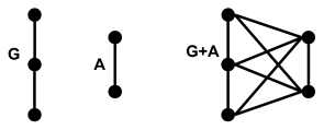
• 1.6.2 Union: given two graphs G and A, their union G∪A creates a disconnected graph with a vertex set V(G)∪V(A) and an edge set V(G)∪V(A).
• 1.6.3 Join: given two graph G and A, their join G+A creates the union of the graphs with the added property that each vertex of G is adjacent to all the vertices of A and each vertex of A is adjacent to all the vertices of G (as such, G+A is a connected graph).
• 1.6.4 Cartesian product: given two graphs G and A, their Cartesian product G⨯A has a vertex set for which every vertex of G⨯A is an ordered pair (u,v) where u∈V(G) and v∈V(A). Two distinct vertices (u,v) and (s,t) within G⨯A are adjacent if either u=s and vt∈E(H) or v=t and us∈E(G). Note that this method of constructing G⨯A requires the vertices of G and A to be labeled in a sequential manner (i.e. V(G)={g₁,g₂,…,g_n} and V(A)={a₁,a₂,…,a_m}) so that equivalences between vertices can be decided. In addition, the Cartesian product of graphs is commutative, that is G⨯A=A⨯G.
• 1.6.5 Transpose: given a digraph D, its transpose is the digraph R such that the direction of each arc in D is reversed.

Definitions [2]

Degrees 2.1

• 2.1.1 Degree: the number of edges incident with a vertex v. This is equivalent to the number of vertices adjacent to v. The degree of v is often denoted as deg(v).
• 2.1.2 Neighborhood: the set N(v) of vertices adjacent to a vertex v.
• 2.1.3 Isolated vertex: a vertex with a degree of zero.
• 2.1.4 Leaf: a vertex with a degree of one, also called an end-vertex.
• 2.1.5 Minimum degree: given a graph G, its minimum degree δ(G) is the lowest degree among the vertices of G.
• 2.1.6 Maximum degree: given a graph G, its maximum degree Δ(G) is the highest degree among the vertices of G.
• 2.1.7 Even vertex: a vertex of even degree.
• 2.1.8 Odd vertex: a vertex of odd degree.
• 2.1.9 Outdegree: for a digraph D, the outdegree od(v) is the number of vertices of D to which v is adjacent.
• 2.1.10 Indegree: for a digraph D, the indegree id(v) is the number of vertices of D from which v is adjacent.
• 2.1.11 Regular graph: a graph with δ(G)=Δ(G) is called regular. For regular graphs, all vertices have the same degree. The degree r of a regular graph’s vertices is used to classify the graph as r-regular.
• 2.1.12 Cubic graph: a graph which is 3-regular.
• 2.1.13 Degree sequence: any list of the degrees found in some graph. Usually, degree sequences can be ordered in multiple ways.
• 2.1.14 Graphical: a finite sequence of nonnegative integers is called graphical if it corresponds to some graph G.

Irregular Graphs 2.2

• 2.2.1 Irregular graph: a graph G with an order of at least two is called irregular if every pair of vertices u∈V(G) and v∈V(G) have distinct degrees.
• 2.2.2 F-degree: for a nontrivial subgraph F⊆G and a vertex v∈G, the F-degree (denoted Fdeg) is the number of copies of F in G which contain v.
• 2.2.3 F-regular: a graph is F-regular if every pair of vertices has the same F-degree.
• 2.2.4 F-irregular: a graph is F-irregular if all pairs of vertices have distinct F-degrees.
• 2.2.5 Underlying graph: if all multi-edges in a multigraph M are replaced by single edges, the resulting graph is called the underlying graph of M.

Matrices and Edge Lists for Graphs 2.3

• 2.3.1 Adjacency matrix: given a graph G of order n, its adjacency matrix A=a_ij is the n x n matrix defined below. Adjacency matrices of simple graphs are symmetric with zeros along the diagonal. Adjacency matrices of pseudographs may have some ones on the diagonal (which indicates self-edges). Adjacency matrices of multigraphs may have integer values greater than one (which indicate more than one edge between given pairs of vertices). Adjacency matrices of digraphs (specifically oriented graphs) are not symmetric (indicating directed edges).

• 2.3.2 Incidence matrix: given a graph G of order n and size m, its incidence matrix B=b_ij is the n x m matrix defined below.

• 2.3.3 Edge list: a list of ordered pairs (u₁,v₁), (u₂,v₂), … , (u_n,u_n) which corresponds to all of the edges in a graph.

Definitions [3]

Isomorphic Graphs 3.1

• 3.1.1 Equal graphs: a pair of graphs with the same vertex set and edge set.
• 3.1.2 Isomorphic graphs: two graphs G and H are isomorphic if there exists a bijective function ϕ which maps V(G) to V(H) such that uv∈E(G) if and only if ϕ(u)ϕ(v)∈V(H). The bijective function ϕ is called an isomorphism. Isomorphic graphs are denoted as G≌H. Isomorphisms are also equivalence relations (and so possess the properties of equivalence relations). Note that isomorphic graphs possess the same structure, but might be drawn differently.
• 3.1.3 Isomorphic digraphs: digraphs D₁ and D₂ are isomorphic if there exists a bijective function ϕ which maps V(D₁) to V(D₂) such that the directed edge (u₁,v₁)∈E(D₁) if and only if (ϕ(u₁),ϕ(v₁))∈E(D₂).
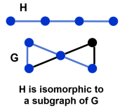
• 3.1.4 Isomorphic to a subgraph: given unlabeled graphs G and H, if for any labeling of the vertices of H and G, the labeled graph H is isomorphic to a subgraph of the labeled graph G.
• 3.1.5 Non-isomorphic graphs: graphs that are not isomorphic, denoted as G≇H.
• 3.1.6 Self-complementary: a graph G which is isomorphic with its complement Ḡ.

Trees 3.2

• 3.2.1 Bridge: consider an edge e=uv of a connected graph G. If removing e from G gives a disconnected graph, then e is a bridge.
• 3.2.2 Acyclic graph: a graph with no cycles. If an acyclic graph consists of more than one component, it is also called a forest.
• 3.2.3 Tree: an acyclic connected graph T.
• 3.2.4 End-vertex: a vertex with a degree of one.
• 3.2.5 Double star: a tree containing exactly two vertices that are not end-vertices.
• 3.2.6 Linear graph: a tree with exactly two end-vertices, also called a path graph.
• 3.2.7 Caterpillar: a tree with an order of at least three for which removal of its end-vertices would give a linear graph. In the case of caterpillars, this linear graph is called a spine.
• 3.2.8 Rooted tree: a tree T for which some vertex v∈T is designated as the root of T. When drawing rooted trees, the root is placed at the top and the other vertices at successively lower levels depending on their geodesic distance from the root.

Minimum Spanning Tree Problem 3.3

• 3.3.1 Spanning tree: given a connected graph G, a spanning tree is a spanning subgraph T⊆G that is also a tree.
• 3.3.2 Minimum spanning tree: given a connected weighted graph G, its minimum spanning tree is the spanning tree T for which the sum of its edge weights is the lowest value among all possible spanning trees of G. Finding a minimum spanning tree of a graph G is called the minimum spanning tree problem.
• 3.3.3 Kruskal’s algorithm: an algorithm for finding a minimum spanning tree T of a connected weighted graph G. To carry out Kruskal’s algorithm, first choose any edge e₁∈G with the minimum weight among the edge set of G and mark e₁ as an edge of T. Then choose another edge e₂∈G with the minimum weight among the remaining edge set of G and mark e₂ as an edge of T. Next, choose a third edge e₃∈G such that adding e₃ into the edge set of T does not create any cycles (e₃ must still possess the minimum weight among the remaining edge set of G) and mark e₃ as an edge of T. Continue this process with each new edge having the minimum weight among the remaining edge set and not creating any cycles until a spanning graph T has been constructed. The resulting graph is a minimum spanning tree of G.
• 3.3.4 Prim’s algorithm: an algorithm for finding a minimum spanning tree T of a connected weighted graph G with order n. To carry out Prim’s algorithm, first choose any vertex v∈G and an edge e₁∈G incident with v such that e₁ has the lowest weight among the edges incident with v. Add this edge to T. Continue adding edges (e₂, e₃, e₄, … , e_n-1) to T such that each edge has the minimum weight among the set of edges that possess exactly one vertex incident with an edge already selected.

Definitions [4]

Connectivity 4.1

• 4.1.1 Cut-vertex: given a connected graph G, if the removal of a vertex v∈G turns G into a disconnected graph, then v is called a cut-vertex. (Note that vertex removal can be denoted by G – v). For a disconnected graph G, cut-vertices are defined as vertices for which removal would turn any component of G into two or more disconnected subgraphs of G (rather than a single disconnected subgraph of G).
• 4.1.2 Nonseparable graph: a nontrivial connected graph which does not contain any cut-vertices.
• 4.1.3 Separable graph: a nontrivial connected graph which contains at least one cut-vertex.
• 4.1.4 Edge-disjoint subgraphs: two subgraphs are called edge-disjoint if they do not share any common edges.
• 4.1.5 Block: for a nontrivial connected graph G which is separable, a block is a nonseparable subgraph H⊆G such that H is not a proper subgraph of any other nonseparable subgraph in G.
• 4.1.6 Vertex-cut: a set of vertices U∈V(G) such that G – U is a disconnected graph.
• 4.1.7 Minimum vertex-cut: a vertex-cut of minimum cardinality in G (cardinality is the number of elements in a set).
• 4.1.8 Vertex-connectivity: the cardinality of a minimum vertex-cut of a graph. Vertex connectivity is also referred to as just connectivity and is denoted by κ(G).
• 4.1.9 k-connected graph: a graph with κ(G)≥k (where k is a nonnegative integer).
• 4.1.10 Edge-cut: a set of edges X∈E(G) such that G – X is a disconnected graph.
• 4.1.11 Minimal edge-cut: an edge-cut X of a connected graph G is called minimal if no proper subset of X is an edge-cut of G.
• 4.1.12 Minimum edge-cut: for an edge-cut X which is not minimal (of a connected graph G), there exists a proper subset Y⊂X that is a minimal edge edge-cut. An edge-cut of minimum cardinality is called a minimum edge-cut. Note that every minimum edge-cut is a minimal edge-cut, but not every minimal edge-cut is a minimum edge-cut.
• 4.1.13 Edge-connectivity: given a nontrivial graph G, the edge-connectivity λ(G) is the cardinality of a minimum edge-cut of G.
• 4.1.14 k-edge-connected graph: a graph with λ(G)≥k (where k is a nonnegative integer), often denoted by K_n.

Terms Relevant to Menger’s Theorem 4.2

• 4.2.1 Separation: a set of vertices S∈G separates two vertices u and v if G – S is a disconnected graph with u and v belonging to different components of G – S. The set S is called a u-v separating set.
• 4.2.2 Minimum u-v separating set: a u-v separating set S with minimum cardinality among all possible u-v separating sets of a graph.
• 4.2.3 Internal vertex: given a u-v path P, an internal vertex of P is a vertex w∈P such that w≠u,v.
• 4.2.4 Internally disjoint paths: a collection of u-v paths {P₁,P₂,…,P_k} such that none of the paths possess common vertices with the exception of the vertices u and v.

Definitions [5]

Eulerian Graphs 5.1

• 5.1.1 Eulerian circuit: a circuit which contains every edge of a graph G.
• 5.1.2 Eulerian graph: a connected graph containing an Eulerian circuit.
• 5.1.3 Eulerian trail: an open trail which contains every edge of a graph G.

Hamiltonian Graphs 5.2

• 5.2.1 Hamiltonian walk: a walk which contains every vertex of a graph G.
• 5.2.2 Hamiltonian cycle: a cycle which contains every vertex of a graph G.
• 5.2.3 Hamiltonian graph: a graph containing a Hamiltonian cycle.
• 5.2.4 Hamiltonian path: a path which contains every vertex of a graph G.
• 5.2.5 Petersen graph: a simple graph with ten vertices and fifteen edges, often used as a counterexample for various graph-theoretic problems.
• 5.2.6 Spanning walk: a walk which visits every vertex of a graph at least once. Note that a Hamiltonian walk is a closed spanning walk of minimum length.

Digraphs 5.3

• 5.3.1 Orientation of a graph: given a simple graph G, the orientation of G is a digraph generated by assigning a direction to each edge of G.
• 5.3.2 Subdigraph: a digraph H such that V(H)⊆G and E(H)⊆G where G is a digraph containing H.
• 5.3.3 Symmetric digraph: a digraph D for which every directed directed edge (u,v)∈G, there also exists a directed edge (v,u)∈G. Note that directed edges are also called arcs.
• 5.3.4 Directed walk: a sequence of vertices starting with u∈G and ending with v∈G such that consecutive vertices are adjacent and the walker proceeds in the direction of the arrows. The length of a directed walk is the number of arcs traversed. If no arc is repeated over a directed walk, then the directed walk is called a directed trail. If no vertex is repeated over a directed walk, then the directed walk is called a directed path.
• 5.3.5 Closed directed walk: a directed walk such that u=v.
• 5.3.6 Open directed walk: a directed walk such that u≠v.
• 5.3.7 Directed circuit: a closed directed trail with a length of at least two.
• 5.3.8 Directed cycle: a closed directed walk with a length of at least two.
• 5.3.9 Directed distance: given a digraph D and vertices u,v∈D, the directed distance d(u,v) is the length of the shortest u-v path in D. As with simple graphs, a u-v path of length d(u,v) is called a geodesic.
• 5.3.10 Weakly connected digraph: a digraph D with a connected underlying graph.
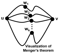
• 5.3.11 Strongly connected digraph: if a digraph D contains both a u-v path and a v-u path for every pair of vertices u,v∈D. An orientation which converts a simple graph into a strongly connected digraph is called a strong orientation. Alternatively, a strongly connected digraph is a digraph for which every vertex can be visited by a single directed path.
• 5.3.12 Eulerian digraph: a digraph containing an Eulerian circuit.

Digraph Tournaments 5.4

• 5.4.1 Tournament: an orientation of a complete graph.
• 5.4.2 Transitive tournament: a tournament T for which the following statement holds. Whenever T has arcs (u,v) and (v,w), it also has an arc (u,w).
• 5.4.3 Directed Hamiltonian path: a path containing all vertices of a digraph D.
• 5.4.4 Directed Hamiltonian cycle: a cycle containing all vertices of a digraph D.
• 5.4.5 Hamiltonian digraph: a digraph D containing a Hamiltonian cycle.

Theorems [1]

• Theorem 1.1: if a graph G with a walk of length L, then G contains a path of length p≤L.
• Theorem 1.2: the vertices and edges of a trail, path, circuit, or cycle in a graph G form a subgraph H⊆G.
• Theorem 1.3: if vertices u and v belong to different components of a disconnected graph, uv∉E(G).
• Theorem 1.4: given a graph G with an order of three or more and two distinct vertices u and v. If u is connected to G and v is connected to G, then G is a connected graph.
• Theorem 1.5: given a connected graph G with an order of three or more, G contains a pair of distinct vertices u and v such that G is connected to u and G is connected to v.
• Theorem 1.6: the size of a complete graph of order n is given by n(n-1)/2.
• Theorem 1.7: if G is a disconnected graph, then its complement Ḡ is connected.
• Theorem 1.8: the nontrivial graph G is a bipartite graph if and only if G does not contain odd cycles.

Theorems [2]

• Theorem 2.1 handshaking lemma: given a graph G with a size of m, the sum of the degrees of the vertices is equal to 2m (or twice the total number of edges).

• Theorem 2.2: every graph has an even number of odd vertices.
• Theorem 2.3: given a graph G of order n and the relation below (in which u and v represent nonadjacent vertices), G is connected and diam(G)≤2.

• Theorem 2.4: given a graph G of order n and δ(G)≥(n-1)/2, the graph G is connected.
• Theorem 2.5: given integers r and n such that 0≤r≤n-1, there exists an r-regular graph of order n if and only if either r or n is even.
• Theorem 2.6: for every graph H and every integer r≥Δ(G), there exists an r-regular graph G which contains H as an induced subgraph.
• Theorem 2.7: a non-increasing sequence of nonnegative integers s₁, s₂, … s_n (where s₁≥1) is graphical if and only if the sequence below is graphical.

• Theorem 2.8: if a graph’s adjacency matrix A=a_ij is raised to a power k, then the entry a_ij^k in row i and column j of A^k is equal to the number of distinct v_i-v_j walks of length k within the graph.
• Theorem 2.9 the party theorem: for any nontrivial simple graph, there exists a pair of vertices with the same degree. As such, no nontrivial simple graph is irregular.
• Theorem 2.10: given a graph F with order k≥2 and a graph G which contains m copies of F as subgraphs, the equality below (involving the F-degree) is true.

• Theorem 2.11: given a subgraph F with an even order and a graph G, the graph G has an even number of vertices with an odd F-degree.
• Theorem 2.12: given a nontrivial connected graph F, there exists an F-irregular graph if and only if Fdeg≠2.
• Theorem 2.13: given a connected graph G with an order of two or more, G is the underlying graph of an irregular multigraph or irregular weighted graph.
• Theorem 2.14 Euler’s formula: given a graph with V vertices, E edges, and F faces (recall that the space outside of a graph is counted as a face) that is drawn without edge intersections, the relation below is always true.

• Theorem 2.15: given an adjacency matrix A of a digraph D, the transposed matrix A^T is the adjacency matrix of a digraph R such that R is the graph transpose of D.

Theorems [3]

• Theorem 3.1: two graphs are isomorphic if and only if their complements are isomorphic.
• Theorem 3.2: two isomorphic graphs G and H possess identical sets of vertex degrees.
• Theorem 3.3: two isomorphic graphs G and H possess the same structural properties. For instance, G is bipartite if and only if H is bipartite, G is connected if and only if H is connected, G contains a 3-cycle if and only if H contains a 3-cycle, etc.
• Theorem 3.4: isomorphism is an equivalence relation on the set of all graphs and so isomorphism is reflexive (every graph is isomorphic to itself), symmetric (there exists an inverse for every isomorphism), and transitive (if G₁≌G₂ and G₂≌G₃, then G₁≌G₃).
• Theorem 3.5: an edge e∈G is a bridge if and only if e does not lie on any cycles of G.
• Theorem 3.6: a graph G is a tree if and only if every pair of vertices in G are connected by a unique path.
• Theorem 3.7: every nontrivial tree has at least two end-vertices.
• Theorem 3.8: every tree of order n has a size of n–1.
• Theorem 3.9: every forest of order n with k components has a size of n–k.
• Theorem 3.10: given a graph G of order n and size, if G satisfies any two of the following properties, then G is a tree. (i) G is connected, (ii) G is acyclic, (iii) m=n–1.
• Theorem 3.11: if T is a tree with order k and G is a graph with minimum degree δ(G)≥k–1, then T is isomorphic to some subgraph of G.
• Theorem 3.12: every connected graph contains at least one spanning tree.

Theorems [4]

• Theorem 4.1: given a vertex v incident with a bridge within a connected graph G, v is a cut-vertex of G if and only if deg(v)≥2.
• Theorem 4.2: given a connected graph G with an order of three or greater, if G contains a bridge, then G contains a cut-vertex.
• Theorem 4.3: given a cut-vertex v in a connected graph G as well as vertices u and w that belong to distinct components of the disconnected graph G – v, the vertex v lies on every u-w path of G.
• Theorem 4.4: a vertex v of a connected graph G is a cut-vertex if and only if there exist vertices u and w (distinct from v) such that v lies on every u-w path of G.
• Theorem 4.5: consider a nontrivial connected graph G and vertices u,v∈V(G). If v is the farthest possible vertex from u as measured by d(u,v), then v is not a cut-vertex of G.
• Theorem 4.6: every nontrivial connected graph contains at least two vertices which are not cut-vertices.
• Theorem 4.7: given a graph G with an order of three or greater, G is nonseparable if and only if every two vertices lie on a common cycle.
• Theorem 4.8: an equivalence relation R can be defined on the edge set of a nontrivial connected graph G for edges e,f∈E(G) when e=f or e and f lie on a common cycle of G.
• Theorem 4.9: every two distinct blocks B₁ and B₂ in a nontrivial connected graph have the following properties. (i) B₁ and B₂ are edge disjoint, (ii) B₁ and B₂ have at most one common vertex, and (iii) if B₁ and B₂ share a common vertex v, then v is a cut-vertex of G.
• Theorem 4.10: for every positive integer n, there exists a k-edge-connected graph K_n such that λ(K_n)=n-1.
• Theorem 4.11: for every graph G, the relation κ(G)≤λ(G)≤δ(G) holds. (Recall that δ(G) denotes a graph’s minimum degree).
• Theorem 4.12: for a cubic graph (3-regular), then κ(G)=λ(G).
• Theorem 4.13: if a graph has order n and size m≥n-1, then κ(G)≤2m/n.
• Theorem 4.14 Menger’s theorem: given nonadjacent vertices u and v in a graph G, the minimum number of vertices in a u-v separating set equals the maximum number of internally disjoint u-v paths in G.
• Theorem 4.15: a nontrivial graph G is k-connected for an integer k≥2 if and only if every pair of distinct vertices u,v∈G corresponds to at least k internally disjoint u-v paths in G.
• Theorem 4.16: given a k-connected graph G any set S of k vertices in G, if a new vertex w is created and joined to the vertices of S, then the resulting graph is also k-connected.
• Theorem 4.17: given a k-connected graph G and vertices k+1 distinct vertices of u,v₁,v₂,…,v_k∈G; there exist internally disjoint u-v_i paths such that 1≤i≤k.
• Theorem 4.18: given a k-connected graph G with k≥2, every k vertices of G lie on a common cycle of G.
• Theorem 4.19: given distinct vertices u and v in a graph G, the minimum number of edges in G which separate u and v equals the maximum number of edge-disjoint u-v paths in G for each pair of distinct vertices u,v∈
• Theorem 4.20: a nontrivial graph G is k-edge-connected if and only if G contains k edge-disjoint u-v paths for each pair of distinct vertices u,v∈G.

Theorems [5]

• Theorem 5.1: a connected graph G contains an Eulerian trail if and only if every vertex of G has an even degree or exactly two vertices of G have odd degrees. In the case of a graph with exactly two vertices of odd degree, each Eulerian trail begins at one of the vertices with an odd degree and ends at the other vertex with an odd degree.
• Theorem 5.2: the Petersen graph is non-Hamiltonian.
• Theorem 5.3: given a Hamiltonian graph G, then every nonempty proper subset S of vertices in G satisfies the relation k(G – S)≤|S|, where k(G – S) is the number of components in the graph G – S and |S| is the cardinality of S.
• Theorem 5.4: if a graph G contains a cut-vertex, then G is not Hamiltonian.
• Theorem 5.5: given a graph G with an order n≥3, if deg(u)+deg(v)≥n for every pair of nonadjacent vertices u,v∈G, then G is Hamiltonian.
• Theorem 5.6: given a graph G with an order n≥3 and deg(v)≥n/2 for every vertex v∈G, then G is Hamiltonian.
• Theorem 5.7: given two nonadjacent vertices u and v in a graph G of order n such that deg(u)+deg(v)n, G+uv is Hamiltonian if and only if G is Hamiltonian. Note that G+uv denotes the graph G with a new edge between vertices u and v (which were formerly nonadjacent).
• Theorem 5.8: given a graph G with an order n≥3, if the relation 1≤j≤n/2 holds for every integer j and the number of vertices in G with a degree of at most j is less than j, then G is Hamiltonian.
• Theorem 5.9 Handshaking lemma for digraphs: given a digraph D with size m and V(D)={v₁,v₂,…,v_n}, the equation below holds.

• Theorem 5.10: if a digraph D contains a u-v walk with a length of L, then D contains a u-v path with a length of at most L.
• Theorem 5.11: a digraph D is strong if and only if D contains a closed spanning walk.
• Theorem 5.12: a nontrivial connected digraph D is Eulerian if and only if od(v)=id(v) for each vertex v∈D.
• Theorem 5.13: a nontrivial connected graph G has a strong orientation if and only if G does not contain any bridges.
• Theorem 5.14: a tournament T is transitive if and only if T does not contain any cycles.
• Theorem 5.15: if u is a vertex with a maximum outdegree for a tournament T, then d(u,v)≤2 for every vertex v∈T.
• Theorem 5.16: every tournament T contains a Hamiltonian path.
• Theorem 5.17: every vertex in a tournament T which is nontrivial and strongly connected belongs to a directed 3-cycle.
• Theorem 5.18: a nontrivial tournament T is Hamiltonian if and only if T is strongly connected.
• Theorem 5.19: given a strongly connected tournament T with an order n≥4, there exists a vertex v such that T – v is also a strongly connected tournament.

Application: methods of proof

New mathematical concepts and tools are made through proofs. Using a series of logical steps, previously unrealized insights about the universe can be uncovered. Existing definitions and theorems are built upon, allowing an ever-expanding system of truth to develop, a system known as mathematics.

• Direct proof: a sequence of statements which starts with a given statement p and ends by proving a statement q. Each successive statement must logically follow from the previous statement.
• Proof by contradiction: by assuming that the negation of a statement q is true and then finding a logical contradiction, q can be proven. Negation is a logical operator denoted as ¬ If ¬q is true, then q is false. If ¬q is false, then q is true.
• Contrapositive proof: the statements p⇒q and ¬p⇒¬q are logically equivalent, so p⇒q can be proven by proving the contrapositive ¬p⇒¬q.
• Proving a biconditional: a logical biconditional is denoted as p⇔q, “p if and only if q,” p⇒q and q⇒p, or “p is necessary and sufficient for q.” Biconditionals can be proven in several ways. (i) By proving p⇒q and q⇒ (ii) By proving p⇒q and ¬p⇒¬q. (iii) By proving ¬q⇒¬p and q⇒p. (iv) By proving ¬q⇒¬p and ¬p⇒¬q.
• Proof by induction: consider a true basis statement p₁ that is true and an infinite sequence of statements p₁⇒p₂⇒p₃⇒…⇒p_n such that each statement logically implies the next in the sequence. If we know that p₁ is true, then all the other statements are also true. To prove by induction, show that p₁ is true and then show that p_n⇒p_n+1 for all n.
• Proof by cases: some proofs can be simplified by breaking the problem into cases and proving each case separately (i.e. proving a statement for even numbers and then for odd numbers).

Application: statistical properties of graphs

Graph theoretic models of complex networks can be analyzed using statistical properties. Such properties are useful for many real-world technological, social, and biological networks. In particular, network properties have revealed insights about the brain and may serve as a quantitative diagnosis method for mental illnesses, neurodegenerative diseases, and other disorders of the nervous system.

• Mean vertex degree: the average degree of vertices in a network.
• Degree distribution: the set of all vertex degrees in a network ordered in a sequential manner (often by increasing degree value). Depending on the particular network, this can result in Gaussian, bimodal, skewed, or other types of distribution.
• Assortativity: a measure of degree correlation between adjacent vertices, often described by an assortativity coefficient r, a Pearson correlation coefficient computed using the degrees of all adjacent vertex pairs in a network. In the formula below (for undirected networks), q_j represents the number of edges incident on a vertex j with the exception of the edge between vertex j and vertex k. Likewise, q_k represents the number of edges incident with a vertex k with the exception of the edge between vertex k and vertex j.

• Clustering coefficient: given a vertex v, its clustering coefficient C is defined as the number of edges s among the set of N vertices adjacent to v over the maximum possible number of edges among said vertices. Note that this measure excludes the edges incident with v itself.

• Mean path length: the average number of vertices traversed by the paths in a network.
• Efficiency: the inverse of a path length L given by 1/L, often used because it is more convenient for certain topological analyses of networks.
• Connection density: given a network of order n, its connection density d (also called cost) is defined as the network’s size S over the size of a complete graph of order n.

• Closeness centrality: a measure of how many shortest paths between all pairs of vertices in a network pass through a given vertex u. The higher the closeness centrality, the closer u is to all other vertices in the network. In the equation below, N is the network’s order and v represents all of the vertices such that v≠u.

• Robustness: describes how much a network’s overall structure and statistical properties are altered upon perturbations like vertex deletions, edge deletions, vertex insertions, edge insertions, reversals of edge directionalities, and changes to edge weight. Robustness can be quantified by a diverse array of methods.
• Modularity: a term describing networks which include densely interconnected subgraphs known as modules. Not many edges are formed between vertices within a given module and vertices outside of said module. Modularity can be quantified by a diverse array of methods.
• Hubs: vertices with high closeness centrality values are called hubs. Alternatively, vertices with high degree can be called hubs.
• Provincial hubs: vertices found inside of modules are often called provincial hubs.
• Connector hubs: vertices which link distinct modules are often called connector hubs.
• Small-worldness: a property proportional to a network’s mean clustering coefficient over its mean path length. Networks with high small-worldness are called small-world networks.

• Scale-free: a network with a degree distribution that is described by a power law is a called scale-free. Power law distributions are defined by the probability mass function P(X=k)=k^-λ where k is the degree of a given vertex in the network and λ is a constant parameter specific to the network under investigation.

Application: the graph Laplacian and random walks

The graph Laplacian (also called the Laplacian matrix) allows a variety of useful analyses to be carried out on graphs. In particular, it can probabilistically describe a random walker’s activities. Random walkers can be thought of as objects which stochastically “jump from vertex to vertex” on a graph.

• Degree matrix: a matrix D with the degrees of a graph G along the diagonal. The remaining entries of D are zeros. For digraphs, the degree matrix may describe either the indegree or the outdegree.
• Laplacian matrix: given a degree matrix D and an adjacency matrix A which describe some graph, the graph’s Laplacian matrix or graph Laplacian is L=D–A.
• Random walk normalized Laplacian: a matrix defined by L^rw=D^-1 The random walk normalized Laplacian can also be computed by L^rw=I_n–D^-1A where I_n is the identity matrix.
• Transition matrix for a random walker: the term D^-1A from the random walk normalized Laplacian represents the transition matrix P for a random walker on a graph G. For a vertex i∈G and the i^th standard basis vector e_i, the vector x=e_iP is a probability vector describing the distribution of a random walker’s possible locations after taking a single step from vertex i. (Note that a probability vector is a vector of values which sum to one and represent probabilities). If q₀ is a probability vector describing the initial distribution of a random walker’s possible locations and q_t is a probability vector describing the distribution of the random walker’s possible locations after t steps, then q_t=q₀P^t.

References

1. Chartrand G, Zhang P. 2013. A First Course in Graph Theory. Dover Publications.
2. Bullmore E, Sporns O. 2009. Complex brain networks: graph theoretical analysis of structural and functional systems. Nat Rev Neurosci 10:186.

     Humans have puzzled over the possibility of an objective moral theory since the dawn of philosophical inquiry. Many argue that morality is socially constructed rather than based in physical laws. Ethical relativists like Foucault (Wilkin, 1999) and sophists like Protagoras (Guthrie, 1969) have proposed that fundamental ethical truths do not exist. Along a similar line of reasoning, Richard Joyce contends that biases imposed by human evolutionary psychology invalidate the concept of fundamental morality since all ethical ideas depend on our evolutionary history (Joyce, 2001). But certain nondualist approaches to cognitive philosophy may provide a new perspective on this notion, a perspective in which ethical truths are both fundamental and relative. I propose that, if consciousness and emotion derive directly from physical processes, then objective morality exists, but continuously varies over space and time.

     For my theory of objective morality, I assume the panpsychist idea that conscious experience is a property of matter, analogous to mass or charge (Seager, 1995). According to this view, specific physical patterns may give rise to specific emotional states in a one-to-one correspondence, making qualia omnipresent. It should be noted that if panpsychism is true, the stochastic flickers of qualia associated with most matter would likely feel primitive enough that they would be unrecognizable by human standards. Next, I apply an authenticity-driven form of existentialism to this panpsychist perspective, allowing physically-encoded emotions to take on intrinsic meaning. In this writing, I exclude “meaninglessness” from existentialism and instead focus on the aspects of existentialism which involve people creating meaning for themselves (Holt, 2012). The distribution of emotional states across the universe may serve as a starting point for a physical description of ethics. By combining panpsychism with physicalism and existentialism, morality can be linked to physics in an objective fashion.

     Despite its past association with metaphysics, panpsychism is rekindling among contemporary thinkers as an explanation for consciousness (Strawson, 2006). Integrated information theory or IIT (Oizumi, Albantakis, & Tononi, 2014) is a mathematical formulation which seeks to quantify consciousness using the information arising from dynamical systems. Galen Strawson has argued that IIT implies panpsychism since all physical structures contain some amount of information (Strawson, 2006). Furthermore, Adam Barrett has proposed modifications to IIT which may help account for fundamental physical interpretations of the universe like quantum field theory (Barrett, 2014). Panpsychic descriptions of reality are reentering philosophical and scientific discourse as new data are acquired and new theoretical interpretations develop.

     But many still find the concept that inanimate objects may possess primitive qualia to be absurd. To counter this presumption, consider a fragment of quartz resting on a ridge. As the sun rises, photons excite the atoms on the crystal’s surface, causing thermal oscillations to propagate into the quartz. This thermal diffusion is modulated by crystallographic defects, causing a heterogeneous distribution of heat inside the rock. As dusk falls, the quartz fragment begins to cool, emitting heat at varying rates across the surface. The particular rates are influenced directly by this quartz specimen’s pattern of internal defects. Next, consider a mouse, also located on the ridge. As the sun rises, photons excite the retinaldehyde molecules in the mouse’s eyes, triggering signal transduction via electrochemical systems. This signal moves into the mouse’s brain, where it propagates through a series of neural pathways, causing a heterogeneous distribution of neural activity. Soon, the signal’s interaction with preexisting brain structures is translated into a motor action; the mouse blinks and looks away from the bright illumination. The particular motor response is modulated by the structural organization of this mouse’s brain at the given time. The quartz and the mouse both receive sensory inputs, process them according to internal properties, and then give motor outputs. Although the rock’s “brain” is much more disorganized and chaotic than the mouse’s brain, it operates by the same basic principles and could plausibly experience a primitive form of consciousness. As such, the possibility of panpsychism cannot be readily dismissed as absurd or metaphysical.

     Another prominent objection to panpyschism arises from brain processes which occur in a subconscious fashion. For instance, activity in the primary visual cortex (V1) does not correlate with conscious visual experience except for a few special cases (Crick & Koch, 1995) (Boyer, Harrison, & Ro, 2005) (Boehler, Schoenfeld, Heinze, & Hopf, 2008). However, the presence of subconscious neural events does not necessarily indicate that the said events are subconscious from the viewpoint of their associated anatomies. Instead, anatomical structures like V1 may experience their own independent qualia. The full informational content of their perceptions may not be transmitted or translated into the brain areas like the prefrontal cortex (PFC) which can be identified with a patient’s sense of self (Mitchell, Banaji, & Macrae, 2005). Of course, some data does transfer into higher brain regions to facilitate processes like vision, but the information undergoes an extensive series of transformations before arriving at the PFC and other regions associated with conscious processing. For this reason, the “unconscious anatomies” objection is insufficient to invalidate panpsychism.

     While existentialism is often linked to both authenticity in developing a personal outlook on life and to a sense of nihilistic meaningless, I use a modified interpretation of existentialism within this essay. I discard the nihilistic component of existentialism and enhance its emotional authenticity to operate in a manner analogous to Cartesian view around the ontology of thought, cogito ergo sum (Murdoch, Cottingham, Descartes, & Stoothoff, 1985). My interpretation of existentialism revolves around idea that emotions possess intrinsic validity in the same way Descartes argued for the intrinsic validity of consciousness. By applying this form of existentialism to physicalist panpsychism, an objective theory of morality gains feasibility.

     My proposed ethical theory does not mean that morality is uniform throughout the cosmos. Equipping the distribution of emotional states or “affective manifold” with existentialism allows for objective morality to continuously vary as informatic patterns change over space and time. Manifolds are mathematical objects which can be informally described as deformed versions of spaces such as the real line, plane, or three-dimensional Euclidean space. Although the affective manifold would not generally exhibit universal emotional uniformity, particular conformations of the manifold may still represent ultimate maxima or minima over all reality. An ultimate maximum may resemble the Buddhist concept of Nirvana, while an ultimate minimum may resemble a hell far worse than any imagined by the world’s religions. These extrema describe states of absolute moral “good” and absolute moral “bad” in a fashion which is fundamentally linked to physics. While this theory connects morality to fundamental processes in the universe, the said morality is also dependent on spatiotemporal coordinates. Ethical truths vary over the affective manifold except when the manifold holds a constant value across the entire cosmos as in the Nirvana and hell cases. In this way, morality may simultaneously take on objective and relative characteristics. Natural law exists, but a given natural law rarely takes on the same form across any two distinct subsets of spacetime.

     As an example, consider a subset of spacetime which includes only a human named Zebadiah during a specified eight-second time interval. Zebadiah feels unjustly underpaid at his job. During the eight-second period, he notices a fifty-dollar bill sitting on the desk of his boss, Enrique. He is alone and could easily snatch the money without consequences. Zebadiah pockets the fifty-dollar bill and does not experience guilt. He feels that this action is morally correct. Inside the spatial bounds of Zebadiah’s brain and the temporal bounds of the eight-second interval, this action is indeed morally correct on a fundamental level. But after the eight seconds have passed, Zebadiah recalls that Enrique’s wife is ill and cannot work, so Enrique is struggling financially. Zebadiah feels a rush of guilt and places the money back on Enrique’s desk. In this new time period, the Zebadiah-specific natural law has changed. Unknown to Zebadiah, Enrique was watching the entire time via a newly-installed security camera. During both time intervals, Enrique feels that Zebadiah is only taking a moral action if he does not steal the money. From an existential viewpoint, all the described perspectives are valid. Panpsychism connects this existentialism to physical processes, supporting moral objectivity on given subsets of the affective manifold.

     Morality is objective, but not absolute except for the specific situations in which the affective manifold is configured in a universally desirable or undesirable manner. Using a physics-based form of panpsychism along with an interpretation of existentialism which grants intrinsic validity to a subject’s emotions, the affective manifold emerges as a possible source of objective ethics. In most distributions of emotional states over the cosmos, ethical truths undergo continuous variation as spatial and temporal coordinates change. In this way, morality can be quite different for distinct persons and even for individual persons at different times. However, it remains an absolute ethical truth that reconfiguring the affective manifold such that all matter in the universe is optimized for generating a supremely positive emotional state represents a morally ideal action. Likewise, reconfiguring the affective manifold to generate a supremely negative emotional state represents an absolute moral wrong. My objective theory of morality may provide a new perspective on the study of ethics and so help to more effectively derive insights around contemporary ethical problems.

References

Barrett, A. (2014). An integration of integrated information theory with fundamental physics. Frontiers in Psychology. Retrieved from https://www.frontiersin.org/article/10.3389/fpsyg.2014.00063

Boehler, C. N., Schoenfeld, M. A., Heinze, H.-J., & Hopf, J.-M. (2008). Rapid recurrent processing gates awareness in primary visual cortex. Proceedings of the National Academy of Sciences, 105(25), 8742 LP-8747. Retrieved from http://www.pnas.org/content/105/25/8742.abstract

Boyer, J. L., Harrison, S., & Ro, T. (2005). Unconscious processing of orientation and color without primary visual cortex. Proceedings of the National Academy of Sciences of the United States of America, 102(46), 16875 LP-16879. Retrieved from http://www.pnas.org/content/102/46/16875.abstract

Crick, F., & Koch, C. (1995). Are we aware of neural activity in primary visual cortex? Nature, 375(6527), 121–123.

Guthrie, W. K. C. (1969). The Sophists. Cambridge University Press.

Holt, K. (2012). Authentic Journalism? A Critical Discussion about Existential Authenticity in Journalism Ethics. Journal of Mass Media Ethics, 27(1), 2–14. http://doi.org/10.1080/08900523.2012.636244

Joyce, R. (2001). The Myth of Morality. Cambridge University Press.

Mitchell, J. P., Banaji, M. R., & Macrae, C. N. (2005). The Link between Social Cognition and Self-referential Thought in the Medial Prefrontal Cortex. Journal of Cognitive Neuroscience, 17(8), 1306–1315. http://doi.org/10.1162/0898929055002418

Murdoch, D., Cottingham, J., Descartes, R., & Stoothoff, R. (Eds.). (1985). Principles of Philosophy. In The Philosophical Writings of Descartes (Vol. 1, pp. 177–292). Cambridge: Cambridge University Press. http://doi.org/DOI: 10.1017/CBO9780511805042.007

Oizumi, M., Albantakis, L., & Tononi, G. (2014). From the Phenomenology to the Mechanisms of Consciousness: Integrated Information Theory 3.0. PLOS Computational Biology, 10(5), e1003588. Retrieved from https://doi.org/10.1371/journal.pcbi.1003588

Seager, W. E. (1995). Consciousness, information, and panpsychism. Journal of Consciousness Studies, 2(3).

Strawson, G. (2006). Realistic monism: why physicalism entails panpsychism.

Wilkin, P. (1999). Chomsky and Foucault on Human Nature and Politics: An Essential Difference? Social Theory and Practice, 25(2), 177–210. Retrieved from http://www.jstor.org/stable/23559137