physics

Notes on Ultrasound Physics and Instrumentation


No Comments

PDF version: Notes on Ultrasound Physics and Instrumentation – by Logan Thrasher Collins

Fundamentals of ultrasound waves

Sound waves such as those in ultrasound are longitudinal waves where particles oscillate backwards and forwards along the wave’s direction of propagation. This forms regions of higher (compression) and lower (rarefaction) density. Sound waves occur through the exchange of kinetic energy from molecular movement with the potential energy from elastic compression and stretching of bonds.

The speed of sound c depends on the medium. For example, in air c = 330 m/s while in water c = 1480 m/s. The frequency of a sound wave depends on the source producing it. Frequency is measured in Hertz (Hz) where 1 Hz = 1 cycle/second. Sound waves with frequencies greater than or equal to 20 kHz are referred to as ultrasound. The wavelength of a sound wave is λ = c/f. It is measured in mm (or other units of length). A sound wave’s phase describes what position the wave starts at within a cycle of oscillation and is measured in degrees or radians. Phase shifts are typically measured relative to a phase of 0° (or 0 rad). A sound wave’s amplitude corresponds to its “loudness” and describes the height of the wave’s peaks (or depth of its troughs). Cosine-based or complex exponential equations can describe sound waves in a similar way as they describe electromagnetic waves. These equations include amplitude as a coefficient, frequency as a factor multiplied by time, and phase shift as a term added to time.

Ultrasound pressure, power, and intensity

A sound wave’s excess pressure is the difference between its peak amplitude and the normal ambient pressure of the medium. When a medium is compressed, the excess pressure is positive and when it is rarified, the excess pressure is negative. In practice, the ambient pressure is often quite low and can be ignored, in which case pressure is used rather than excess pressure. Excess pressure and pressure are measured in Pascals (Pa), which are equivalent to N/m2.

When an ultrasound wave passes through a medium, it deposits energy (measured in Joules) into said medium. The rate at which a source produces this energy is the power, which is measured in Watts or J/s. An ultrasound wave’s power is unevenly distributed across the beam and often is more concentrated near the beam’s center. Intensity is a measure of the power flowing through a unit area perpendicular (or normal) to the wave’s direction of propagation and is measured in W/m2 or W/cm2. Intensity is proportional to the wave’s pressure squared (I ∝ p2).

Ultrasound and its medium

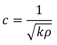
As mentioned, the medium (material) an ultrasound wave passes through determines the sound’s speed of propagation. Specifically, the material’s density and stiffness determine the speed of sound propagation. Density ρ is often measured in kg/m3. For instance, bone’s density ρbone = 1850 kg/m3 and water’s density ρwater = 1000 kg/m3 (or 1 g/cm3). Stiffness k describes how much a material resists deformation by force F. It equals the amount of pressure (stress) needed to change the thickness of a material by a given fraction and is measured in Pa. The ratio of change in thickness ΔL over original thickness L0 is called tensile strain ε. The increase (or decrease) in length of a material due to applied force is denoted ΔL = L – L0. Stress σ or fractional change in thickness is given by change in thickness divided by original thickness of the sample. Stress over strain is the elastic modulus E (also called Young’s modulus). Here, A is the cross-sectional area of a sample perpendicular to the applied force. Note that these formulas apply only for tensile stress (which induces tensile strain), the type of stress where a material is compressed or elongated.

The relationship between a sound wave’s speed and the properties of density and thickness can be modeled by masses on springs where ρ = m = density (corresponding to masses in the model) and k = stiffness (corresponding to the spring stiffness in the model). The relationship between c, ρ, and k is given by the following equation.

As a result of these properties, the speed of sound varies in different tissues. A table of the approximate speeds of sound across selected tissues is provided.

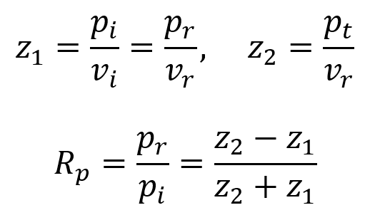
Acoustic impedance z measures the response of a medium’s particles in terms of their velocity v to a sound wave of a given pressure p. Acoustic impedance can also be expressed in terms of density and stiffness or in terms of density and the sound’s speed. The latter form of definition is called the characteristic acoustic impedance of the tissue. It has units of kg m–2 s–1, also called rayl.

Ultrasound reflection and refraction

When an ultrasound wave traveling through a medium of acoustic impedance z1 encounters a new medium of different acoustic impedance z2, some of the wave is transmitted and some is reflected back. The equations in the following discussion will initially assume that the wave approaches the interface at a 90° angle (perpendicular) until stated otherwise.

To maintain continuity across the interface, the following equations must hold. Here, pi and vi are initial pressure and velocity, pr and vr are reflected pressure and velocity, and pt and vt are transmitted pressure and velocity.

Additionally, the intensity transmitted It across the interface equals the incident intensity Ii minus the reflected intensity Ir.

By using the equation for the definition of acoustic impedance z = p/v, the following two equations are true. Algebraically manipulating these equations leads to the third equation below. Rp is called the amplitude (or pressure) reflection coefficient of the interface. It is important because it decides the amplitude of the echoes produced at various interfaces within the tissue.

Note that if the acoustic impedance of the first medium is greater than the acoustic impedance of the second medium (i.e. z1 > z2), then Rp is negative and the reflected wave is inverted (across the x axis). For most interfaces between soft tissues, Rp is quite small and so most of the wave is transmitted to produce further echoes deeper within the tissue. This is useful for ultrasound imaging. Since the interface between air and soft tissue has a much larger Rp, the ultrasound source must be placed in direct contact with the patient’s skin to avoid air blocking transmission. This also means that gas-containing tissues like lungs and gut effectively block imaging beyond the region with the gas.

Another way to describe reflection is in terms of the intensity reflection coefficient RI. Since I ∝ p2, this means that RI = Rp2.

Since the incident intensity is Ii = It + Ir and the transmitted intensity is It = Ii – Ir, one can also define an intensity transmission coefficient TI as the first equation below. Since the transmitted pressure is pt = pi + pr, one can also define a pressure transmission coefficient Tp as the second equation below.

It is useful to realize that, because energy at interfaces must be conserved, the following equation holds true.

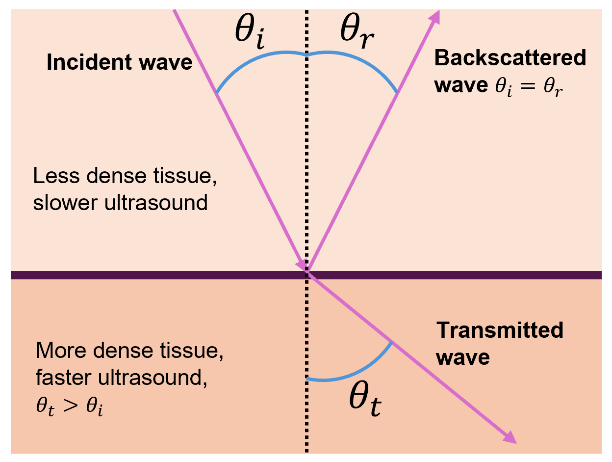
But ultrasound waves often do not approach interfaces at a 90° angle, so the equations in this section must be modified via trigonometry to account for other angles. First, note that the incident angle θi will equal the backscattered angle θr (this is true in the 90° case as well).

When a sound wave in a less dense tissue (slower sound wave) crosses into a tissue of greater density (faster sound wave), the transmitted wave bends away from the normal and thus θt > θi

Likewise, when a sound wave in a tissue of greater density (faster sound wave) crosses into a tissue of less density (slower sound wave), the transmitted wave bends towards the normal and thus θt < θi.

Ultrasound scattering

When ultrasound encounters an object which is small compared to the wavelength, it scatters in all directions, though slightly more energy is typically backscattered towards the transducer than away from it. Scattering specifics depend on the shape, size, and acoustic properties (z, k, ρ) of the object.

When many similar small objects are close together (e.g. red blood cells), constructive interference can occur, which is useful. In the case of the blood, this is the basis for Doppler ultrasound, which measures blood flow. By comparison, when many small objects are far apart, complex interference patterns occur. This leads to a phenomenon in images known as “speckle”, which is usually (but not always) considered a form of undesirable noise.

Absorption and relaxation of ultrasound

As ultrasound moves through tissue, it loses energy due to absorption, resulting in heat. There are two ways this occurs: relaxation absorption and classical absorption. The effects of relaxation absorption are typically much more dominant.

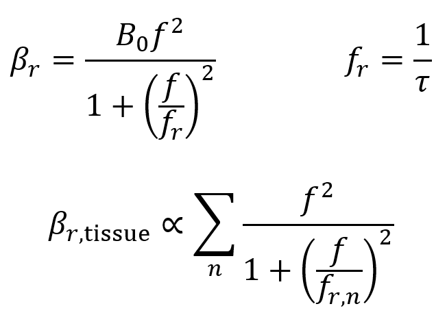
Relaxation absorption depends on the elastic properties of tissue, occurring when the tissue returns to its original state after rarefaction or compression by ultrasound. This is quantified by the relaxation time τ = 1/fr, which is how long the tissue takes to return to its original state after the ultrasound’s effect. 

Relaxation is characterized by a relaxation absorption coefficient βr which is given by the first two equations below. Here, fr is the frequency of relaxation, f is the frequency of ultrasound, and B0 is a material-specific constant. In practice, tissues contain a range of values of τ and fr, so the third equation below is a more general formula where the overall relaxation absorption coefficient is proportional to the sum of the various contributions. Higher values of βr mean more energy is absorbed into the tissue.

It is useful to note that in tissues, the relationship between the relaxation absorption coefficient βr and the frequency f is approximately linear.

Classical absorption is less important in tissues since, at clinical frequencies, the relaxation absorption is strongly dominant as mentioned. That said, overall absorption does consist of a combination of relaxation and classical absorption (though the latter may be approximated away sometimes). Classical absorption occurs because of friction between particles as they are displaced by ultrasound, causing loss of energy to heat. This loss is characterized by the classical absorption coefficient βclass ∝ f2.

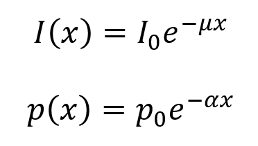
Attenuation coefficients

When an ultrasound beam propagates through tissue, the sum of the absorption and scattering is described as attenuation, which causes an exponential decrease in the pressure and intensity of the ultrasound as a function of the propagation distance x through tissue.

The following equations describe the loss of ultrasound intensity and pressure as the wave moves through tissue. Here, µ is the intensity attenuation coefficient and α is the pressure attenuation coefficient. The value of µ is equal to twice the value of α (so, µ = 2α). Both have units of cm–1, though the value of µ is often given in units of decibels (dB) per cm, where the conversion factor is µ(dB cm–1) = 4.343µ(cm–1). It is useful to note that each 3 dB decrease corresponds to a decrease in intensity by a factor of 2.

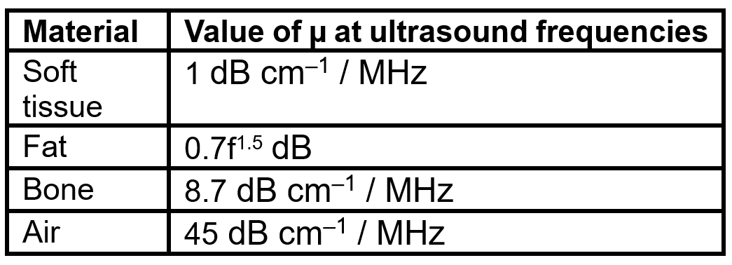
Approximate frequency dependences of µ are given in the table below. As an example, in soft tissue, the value of µ = 1 dB cm–1 for 1 MHz ultrasound and µ = 2 dB cm–1 for 2 MHz ultrasound. Note that the value of µ for fat is calculated differently than the others via the equation µ(f) = 0.7f1.5 dB.

Ultrasound transducers

Ultrasound imaging is performed using ultrasound transducers. A gated frequency generator first produces short periodic voltage pulses, which are then amplified and fed into the transducer via a transmit-receive switch. Because the transducer transmits high power pulses and receives low intensity signals from the reflected ultrasound waves, the transmit and receive circuits must be isolated from each other. Amplified voltage is converted by a shaped piezoelectric material (typically lead zirconate titanate, which is abbreviated PZT) in the transducer into a mechanical pressure wave which is transmitted into the tissue. 

After reflecting and scattering from boundaries within the tissue, pressure wave signals return to the transducer and are converted back into voltages by the piezoelectric material. The voltages must pass through low-noise preamplifier before digitization. Further amplification and signal processing facilitates display of images on a computer.

When oscillating voltage is applied to one end of shaped PZT material, the thickness of the PZT element oscillates at the same frequency as the voltage. By placing this element in contact with skin, mechanical pressure waves are transmitted into tissue. The element has a resonant frequency f0 which is determined by its thickness T and the speed of the ultrasound wave in the PZT material cPZT. The value of cPZT is ~4000 m/s.

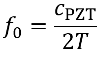
For most ultrasound devices, the transducer element’s thickness must be designed to equal one half the wavelength of ultrasound in the PZT material λPZT, so T = λPZT/2. This facilitates use of the resonant frequency.

Because of the much higher acoustic impedance of PZT material compared to skin (~18 times higher), a large amount of the energy would be reflected if the PZT was placed directly onto the skin’s surface. This would mean the mechanical wave traveling into the tissue would lose most of its energy.

To prevent this energy loss from happening, transducers possess a matching layer with a zmatching value between zskin and zPZT as given by the equation below. The thickness of the matching layer is typically made to be 1/4 of the ultrasound’s wavelength in its material T = λmatching/4. All this improves the transmission and reception efficiency. Sometimes multiple matching layers are used to further improve efficiency.

At the back of a PZT element, there is a damping layer, typically made of some backing material and epoxy. This damping layer prevents the PZT from continuing to oscillate (at a decaying rate) after each voltage pulse. This continued oscillation would blur the boundaries between the short pulses, which can decrease axial resolution (as will be described soon).

Although transducers have a central frequency f0, they typically cover a range of frequencies (e.g. a 3 MHz transducer might cover a range of 1-5 MHz). Higher mechanical damping leads to broader transducer bandwidth. Transducer bandwidth is described as the frequency range over which the sensitivity is greater than half the maximum sensitivity level. The relationship between bandwidth and f0 is often quantified by the quality factor Q, which is the ratio of f0 to the bandwidth. Low values of Q mean larger bandwidths. Note that 2f0 is the second harmonic frequency.

Beam geometry and resolution

FUS transducers produce a very complicated wave pattern close to the face of the transducer (the near-field or Fresnel zone). This complicated pattern is not usually useful since it has many parts where the intensity is zero. Beyond the near-field zone, the wave pattern is much simpler and decays exponentially with distance (the far-field or Fraunhofer zone). The boundary between the two zones is called the near-field boundary (NFB) and occurs at a distance ZNFB away from the face of the transducer. The following equation (where r is the radius of the transducer) can be used to calculate the ZNFB value.

After the NFB, the FUS beam diverges (spreads out laterally) with an angle of deviation θ which is given by the equation below.

For the far-field zone, the lateral shape of the beam approximates a Gaussian function. The full width at half maximum (FWHM) defines the lateral resolution of the beam. It is given by the equation below, where σ is the standard deviation of the Gaussian. This value is unique to each FUS beam at the specific desired depth. It can be calculated by the following equation.

Single element transducers also produce ultrasound side lobes where the first zero of the side lobe at angle φ is the same equation as the FUS beam’s divergence angle equation. In ultrasound imaging, the side lobes can cause artifacts if they are backscattered from tissue outside of the imaged region.

Axial resolution is the closest distance two boundaries can be relative to each other (in a direction parallel to the FUS beam’s propagation) while still allowing them to be resolved as two distinct features. It is given by the equation below where pd is the pulse duration and c represents the speed of the ultrasound in the tissue.

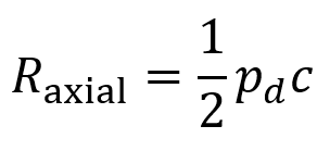
The reason that axial resolution works this way is because the echoes of beams returning from two different boundaries are distinguishable so long as these boundaries are spaced widely enough that they do not overlap in time.

Some typical values of axial resolution are 1.5 mm at a frequency (1/c) of 1 MHz or 0.3 mm at a frequency of 5 MHz. But it should be noted that attenuation of the FUS increases at higher frequencies, so there is an important tradeoff between penetration depth and axial resolution. (Very high frequencies such as 40 MHz can be used for imaging the skin at high resolution).

Single flat ultrasound transducers possess relatively poor lateral resolution. Concave curved transducers can achieve better resolutions. (It should be noted that the transducer equations above may be somewhat altered in the case of curved transducers rather than flat transducers). To make a curved transducer, one can add a curved plastic lens in front of the piezoelectric element or the piezoelectric element itself can be made in a concave curved shape.

The shape of a transducer’s curvature can be described by an “f-number”, which is a value equal to the focal distance divided by the aperture dimension where the aperture dimension is determined by the size of the transducer element.

Lateral resolution for a bowl-shaped curved (focused) transducer is calculated using the following equation below where λ is the ultrasound wavelength, F is the focal distance, and D is the diameter of the transducer. The focal distance F is where the lateral beamwidth is narrowest and is approximated as the radius of curvature (ROC) of the lens or PZT element. This approximation is valid except in the case of very high curvature.

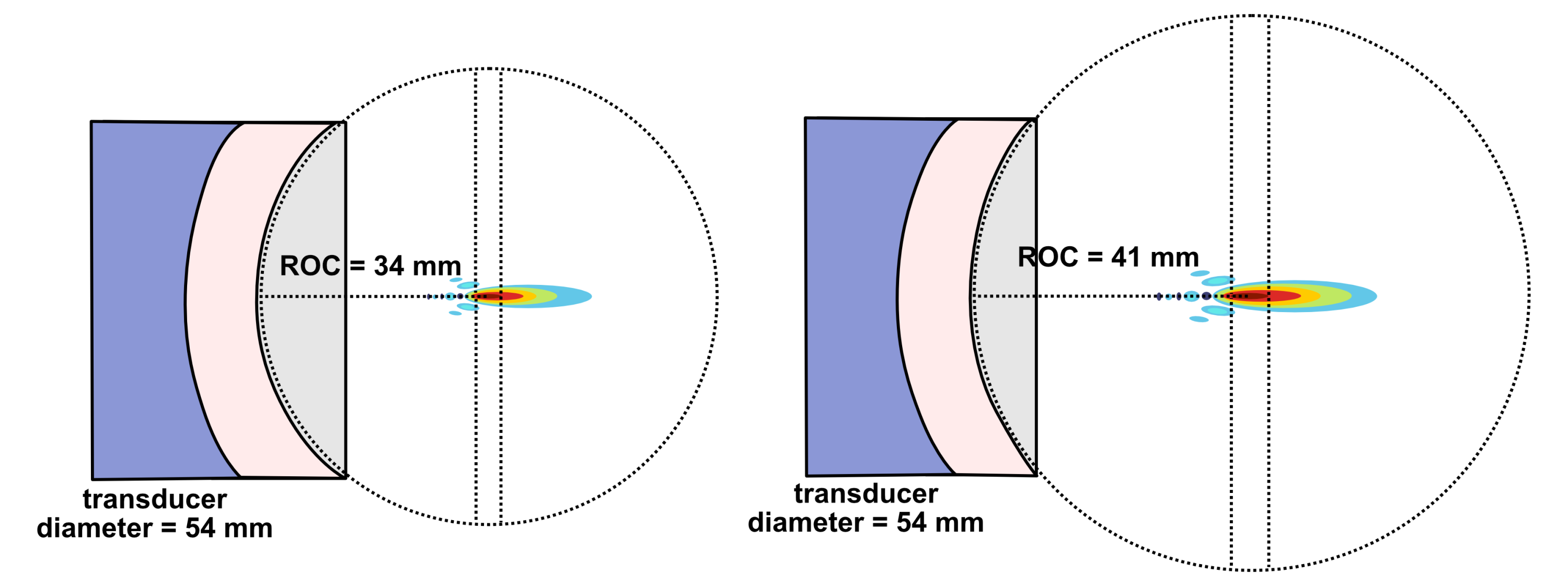
When deciding on the focusing power of a transducer, there is a compromise between high spatial resolution and depth over which good spatial resolution is achievable. For a strongly focused transducer, locations further away from the beam’s focal plane diverge more sharply than for a weakly focused transducer. This can be quantified by the on-axis depth-of-focus (DOF) which equals the axial distance over which the beam’s intensity is at least 50% of its maximum value.

Transducer arrays

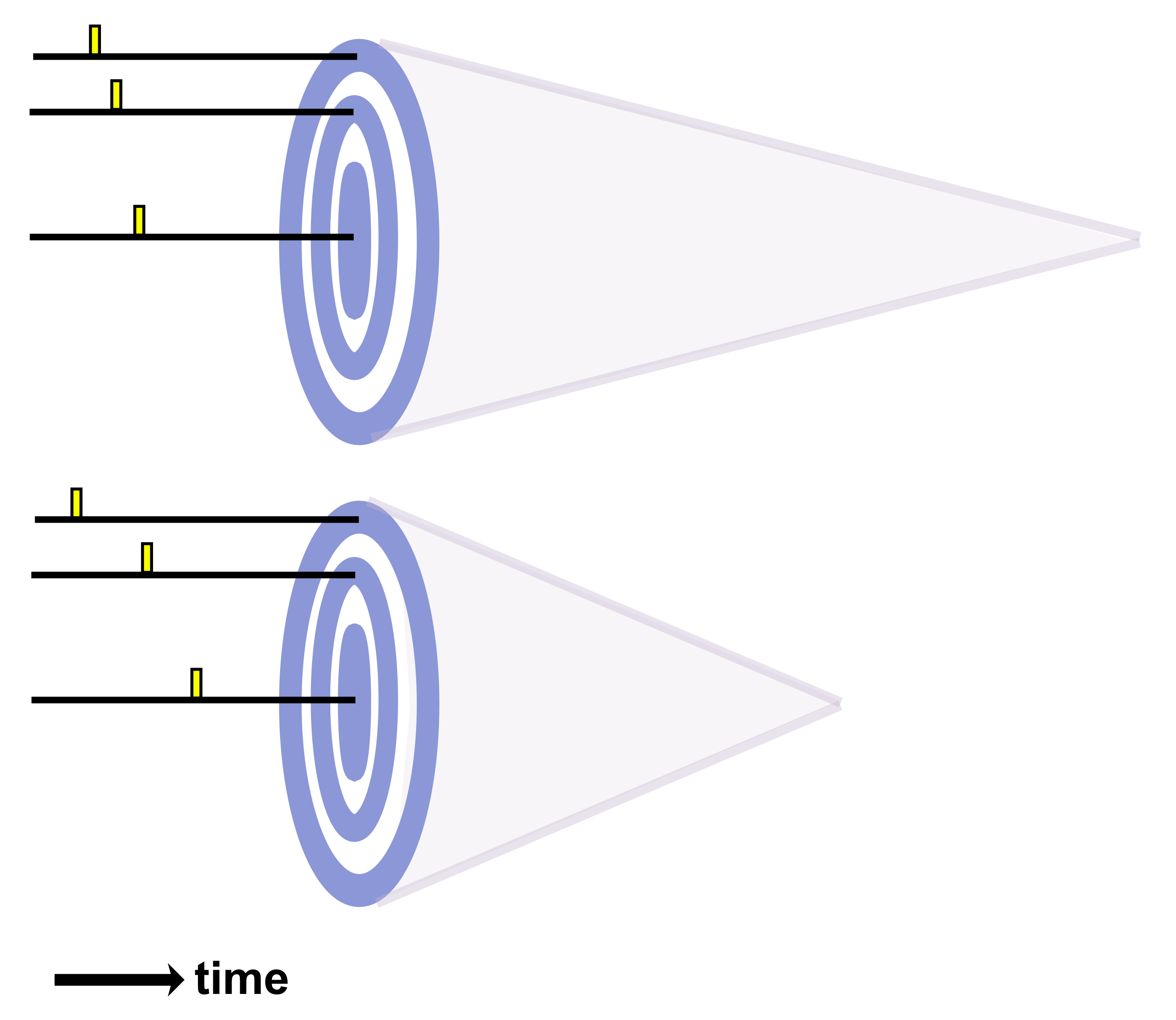
Contemporary FUS systems typically use arrays consisting of many small piezoelectric elements (rather than single-element transducers). These arrays allow 2D imaging via electronic steering of the beam through tissue while the transducer is held at a fixed position. Sophisticated electronics produce a dynamically changing focus during pulse transmission and signal reception, which maintains high resolution throughout the image. Linear and phased array transducers represent the two main types of arrays.

A linear array consists of many (often 128-512) rectangular piezoelectric elements where the space between elements is called kerf and the distance between their centers is referred to as pitch. Each element is mechanically and electrically isolated from its neighbors by filling the kerf regions with acoustically isolating material. The elements are not focused. Pitch is designed to range from λ/2 to 3λ/2 (where λ is ultrasound wavelength in tissue). Linear arrays are usually about 1 cm wide and 10-15 cm long.

Linear arrays work by using separate voltage pulses to excite a small number of elements at slightly different times where the outer elements are excited first and the inner elements are excited after a short delay. This creates an effectively curved wavefront with a focal point at a certain distance from the array. After all backscattered echoes have been received, another beam consisting of a distinct subset of elements performs the same steps. This is repeated in sequence until all of the groups of elements have completed the procedure. If even numbers of elements were used for each group, the entire process can be repeated again with odd numbers of elements to cover the focal points between those acquired before.

Linear array focusing occurs only in one dimension. By contrast, the elevation plane (the direction perpendicular to the image plane) cannot be focused unless a curved lens is included to produce focus in this dimension. Linear arrays are most often used for applications involving large fields of view and relatively low penetration depth.

Phased arrays are typically around 1-3 cm in length and 1 cm in width. They are used in applications like cardiac imaging where there is only a small region of the body through which the ultrasound can enter without running into bone or air.

As with linear arrays, phased arrays apply voltage pulses at slightly varying times to excite elements and produce an effective wavefront with a certain focal length. But phased arrays must employ beam steering to reconstruct a full 2D image. This occurs by changing the pattern of excitation to sweep the effective wavefront beam across a range of directions to cover the image plane.

Phased arrays also employ a process called dynamic focusing to optimize lateral resolution over the full depth of imaged tissue. This involves dynamically changing the number of elements used to produce a wavefront with varying focal lengths. At deeper regions in the tissue, the number of elements needed to position the focus (where optimal lateral resolution is achieved) is higher than at shallower regions in the tissue. Dynamic focusing allows high lateral resolution across the full depth of the scan. However, dynamic focusing is relatively slow since multiple scans are needed to build up a single line of the image. It should be noted that the length of each element determines the “slice thickness” for the image’s elevation dimension.

There are also multidimensional transducer arrays which include extra rows of transducer elements. These multidimensional arrays can focus in the elevation dimension without the need for curved elements or lenses (though they are more complicated devices). Multidimensional arrays with a small number of extra rows (e.g. 3-10) are referred to as 1.5 dimensional arrays. These 1.5D arrays can facilitate some level of focusing in the elevation dimension, though to a limited extent. When multidimensional arrays possess a large number of extra rows (up to the number of elements in each row), they are referred to as 2 dimensional arrays. These can acquire full 3D image data without needing to be moved from their initial position.

Annular arrays represent another class of transducer array. They are useful at very high frequencies (>20 MHz) since linear or phased arrays are quite difficult to create for these frequencies. Annular arrays consist of concentric rings of piezoelectric material alternating with rings acoustically isolating material. Beam forming is accomplished using an analogous strategy to that of phased arrays. The outermost rings are excited first and the innermost rings last, producing an effective focus. Because annular arrays require mechanical motion to sweep the beam through tissue for reconstruction of images, commercially available devices have been developed to precisely control this motion.

When transducer arrays receive signals, they pass through an amplifier to strengthen them before digitization. However, such amplifiers do not provide linear gain for signals with a dynamic range that exceeds 40-50 dB. This is an issue because very strong signals appear from tissue boundaries near the transducer while much weaker signals appear from tissue boundaries deeper in the body. Weak signals can thus be lost when attempting to receive over larger dynamic ranges. A process called time-gain compensation (TGC) is employed to circumvent this issue. TGC increases the amplification factor as a function of time after transmission of an ultrasound pulse. As a result, the weaker backscattered echoes which come later are amplified to a greater degree than the stronger backscattered echoes which come sooner. TGC is controlled by the operator of the instrument, which usually comes with a variety of preset values for clinical imaging protocols.

Parameters for focused ultrasound in practice

There is no universally accepted definition of FUS dose, so various metrics of exposure are used to quantify how much ultrasound is delivered during a therapeutic session. Examples of such metrics (which will be discussed further below) include acoustic pressure or peak negative pressure, mechanical index, frequency, pulse repetition frequency (PRF), and intensity.

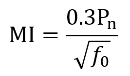
Peak negative pressure is often measured in MPa and describes the degree of rarefaction caused by the ultrasound wave in tissue. For low intensity focused ultrasound (LIFU), the greatest mechanical safety risk is from cavitation (bubble formation and collapse). To measure cavitation risk, the mechanical index (MI) is used. MI can be computed using the following equation where Pn is the peak negative pressure, f0 is the fundamental frequency, and the derating constant of 0.3 adjusts for tissue attenuation (~7% loss per cm per MHz) and has units dBcm–1MHz–1. After derating, 0.3Pn has units of MPa. FDA guidelines specify that MI should not exceed 1.9. MI itself is unitless.

An ultrasound wave’s pulse’s duration (PD) is the number of cycles divided by the frequency. For instance, a pulse with 500 cycles of 500 kHz ultrasound would last for 1 ms. The pulse repetition interval (PRI) is the amount of time between the start of one pulse and the start of the next pulse (so it includes both the pulse and the pause after the pulse). Pulse repetition rate (PRR) also known as the pulse repetition frequency (PRF) equals 1/PRI. The pulse duty cycle (PDC) equals PD/PRI and is expressed as a percentage. PD typically ranges from microseconds to seconds, PRI from milliseconds to seconds, and PDC from <1% up to 70%.

One’s choice of a particular PD and PDC comes from two main factors: (i) the duty cycle can have varying neuromodulatory effects (excitatory or inhibitory) depending on its value and (ii) lower PDC values can be leveraged to limit total energy and heat deposition.

A pulse train is a series of pulses, for which the pulse train duration (PTD) equals the total number of pulses times the PRI. Typical PTDs range from less than 1 second to several minutes. The amount of time between the start of one pulse train and the start of the next is called the pulse train repetition interval (PTRI). The amount of time between pulse trains is called the interstimulus interval (ISI). The pulse train duty cycle (PTDC) equals PTD/PTRI.

It should be noted that the PTDC does not have a major influence on neuromodulatory effect, so the ratio is driven by safety such that the ISI is long enough to limit cumulative heating to reasonable levels.

Multiplying PDC by PTDC gives an overall duty cycle equal to (PD/PRI)(PTD/PTRI) which can be further multiplied by the average intensity of the pulses Iavg to obtain average temporal intensity Iavg_tp. FDA diagnostic safety guidelines state that average intensity should fall below 720 mW/cm2. So, Iavg_tp = (PD/PRI)(PTD/PTRI)Iavg generally should not exceed 720 mW/cm2.

Total ultrasound application time is the sum of the durations of all pulse trains plus ISIs. It typically ranges from less than 1 minute to over 60 minutes. Longer total ultrasound application time is thought to usually improve efficacy by depositing more energy, though this may not always be true. Energy per unit time might play a more significant role in efficacy, but this is an ongoing area of investigation.

Frequency (or fundamental frequency f0) is the primary frequency of FUS passing through the tissue. It is typically measured in kilohertz (kHz) or megahertz (MHz). In human neuromodulation applications, frequency typically ranges from 200-700 kHz (or 0.2-0.7 MHz), providing an acceptable tradeoff between amount of energy entering the brain and the size of the focal region. The reason that the upper limit of frequency for human neuromodulation is typically ~700 kHz is because FUS energy attenuation by the skull at 700 kHz is ~75% (though this varies depending on skull morphology) and keeps increasing at higher frequencies.

Recall from the equations in the earlier discussion that lateral resolution involves wavelength λ (and f = c/λ), so frequency influences the focal region’s size. Also discussed earlier, frequency influences the distance from the transducer to the near-field boundary (ZNFB). Frequency itself is generally not believed to contribute to neuromodulatory effects in a direct fashion, though this is still under investigation. So, the f0 value is usually selected to create a focal volume of a desired size at a given depth.

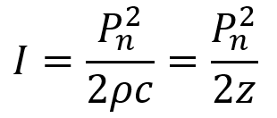
Intensity is defined as power per unit area (and recall the unit of power is Watts or J/s) and is the rate at which energy is transferred by the FUS wave. For ultrasound at any given point in time during the wave cycle, intensity is proportional to the square of the acoustic pressure as described by the equation below where P is the acoustic pressure, ρ is the density of the medium, and c is the ultrasound speed in the medium. Recall that ρc = z, the acoustic impedance. Acoustic intensity is usually measured in watts per square centimeter (W/cm2).

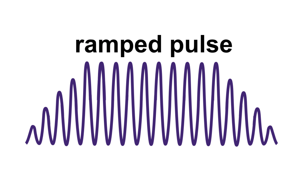
Beyond instantaneous intensity, FUS is often measured by spatial peak pulse average intensity (ISPPA) and by spatial peak temporal average intensity (ISPTA). ISPPA is the average intensity experienced during a single ultrasound pulse. Note that I does not equal Pn2/2z in the case of a ramped pulse. To determine average intensity (ISPPA) for ramped pulses, the integral of intensity across the pulse is divided by the pulse’s duration PD. Ramped pulses distribute energy more smoothly and help mitigate auditory confounds for LIFU applications.

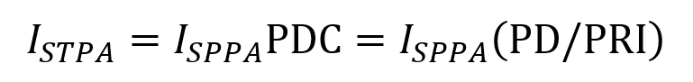
ISPTA represents the average intensity of the FUS beam at the point where it is strongest averaged over the pulse duration while accounting for any off periods. It is described by the following equation consisting of the ISPPA multiplied by the PDC (which is the fraction of PRI that the pulse is turned on).

References:

1.      Legon, W. & Strohman, A. Low-intensity focused ultrasound for human neuromodulation. Nat. Rev. Methods Prim. 4, 91 (2024).

2.      Smith, N. B. & Webb, A. Introduction to Medical Imaging: Physics, Engineering and Clinical Applications. (Cambridge University Press, 2010).

Notes on Quantum Mechanics


No Comments
PDF version: Notes on Quantum Mechanics – By Logan Thrasher Collins

The Schrödinger equation and wave functions

Overview of the Schrödinger equation and wave functions

Quantum mechanical systems are described in terms of wave functions Ψ(x,y,z,t). Unlike classical functions of motion, wave functions determine the probability that a given particle may occur in some region. The way that this is achieved involves integration and will be discussed later in these notes.

To find a wave function, one must solve the Schrödinger equation for the system in question. There are time-dependent and time-independent versions of the Schrödinger equation. The time-dependent version is given in 1D and 3D by the first pair of equations below and the time-independent version is given in 1D and 3D by the second pair of equations below. Here, ћ is h/2π (and h is Planck’s constant), V is the particle’s potential energy, E is the particle’s total energy, Ψ is a time dependent wave function, ψ is a time-independent wave function, and m is the mass of the particle. After this point, these notes will focus on 1D cases unless otherwise specified (it will often be relatively straightforward to extrapolate to the 3D case).

For a wave function to make physical sense, it needs to satisfy the constraint that its integral from –∞ to ∞ must equal 1. This reflects the probabilistic nature of quantum mechanics; the probability that a particle may be found anywhere in space must be 1. For this reason, one must usually find a (possibly complex) normalization constant A after finding the wave function solution to the Schrödinger equation. This is accomplished by solving the following integral for A. Here, Ψ* is the complex conjugate of the wave function without the normalization constant and Ψ is the wave function without the normalization constant.

To obtain solutions to the time-dependent Schrödinger equation, one must first solve the time-independent Schrödinger equation to get ψ(x). The general solution for the time-dependent Schrödinger equation is any linear combination of the product of ψ(x) with an exponential term (see below). The coefficients cn can be real or complex.

Physically, |cn|2 represents the probability that a measurement of the system’s energy would return a value of En. As such, an infinite sum of all the |cn|2 values is equal to 1. In addition, note that each Ψn(x,t) = ψn(x)e–iEnt/ is known as a stationary state. The reason these solutions are called stationary states is because the expectation values of measurable quantities are independent of time when the system is in a stationary state (as a result of the time-dependent term canceling out).

Using wave functions

Once a wave function is known, it can be used to learn about the given quantum mechanical system. Though wave functions specify the state of a quantum mechanical system, this state usually cannot undergo measurement without altering the system, so the wave function must be interpreted probabilistically. The way the probabilistic interpretation is achieved will be explained over the course of this section.

Before going further, it will be useful to understand some methods from probability. First, the expectation value is the average of all the possible outcomes of a measurement as weighted by their likelihood (it is not the most likely outcome as the name might suggest). Next, the standard deviation σ describes the spread of a distribution about an average value. Note that the square of the standard deviation is called the variance.

Equations for the expectation value and standard deviation are given as follows. The first equation computes the expectation value for a discrete variable j. Here, P(j) is the probability of measurement f(j) for a given j. The second equation is a convenient way to compute the standard deviation σ associated with the expectation value for j. The third equation computes the expectation value for a continuous function f(x). Here, ρ(x) is the probability density of x. When ρ(x) is integrated over an interval a to b, it gives the probability that measurement x will be found over that interval. The fourth equation the same as the second equation, but finds the standard deviation σ for the continuous variable x.

In quantum mechanics, operators are employed in place of measurable quantities such as position, momentum, and energy. These operators play a special role in the probabilistic interpretation of wave functions since they help one to compute an expectation value for the corresponding measurable quantity.

To compute the expectation value for a measurable quantity Q in quantum mechanics, the following equation is used. Here, Ψ is the time-dependent wave function, Ψ* is the complex conjugate of the time-dependent wave function, and Q̂ is the operator corresponding to Q.

Any quantum operator which corresponds to a classical dynamical variable can be expressed in terms of the momentum operator –iℏ(∂/∂x). By rewriting a given classical expression in terms of momentum p and then replacing every p within the expression by –iℏ(∂/∂x), the corresponding quantum operator is obtained. Below, a table of common quantum mechanical operators in 1D and 3D is given.

Heisenberg uncertainty principle

The Heisenberg uncertainty principle explains why quantum mechanics requires a probabilistic interpretation. According to the Heisenberg uncertainty principle, the more precisely the position of a particle is determined via some measurement, the less precisely its momentum can be known (and vice versa). The Heisenberg uncertainty principle is quantified by the following equation.

The reason for the Heisenberg uncertainty principle comes from the wave nature of matter (and not from the observer effect). For a sinusoidal wave, the wave itself is not really located at any particular site, it is instead spread out across the cycles of the sinusoid. For a pulse wave, the wave can be localized to the site of the pulse, but it does not really have a wavelength. There are also intermediate cases where the wavelength is somewhat poorly defined and the location is somewhat well-defined or vice-versa. Since the wavelength of a particle is related to the momentum by the de Broglie formula p = h/λ = 2πℏ/λ, this means that the interplay between the wavelength and the position applies to momentum and position as well. The Heisenberg uncertainty principle quantifies this interplay.

Some simple quantum mechanical systems

Infinite square well

The infinite square well is a system for which a particle’s V(x) = 0 when 0 ≤ x ≤ a and its V(x) = ∞ otherwise. Because the potential energy is infinite outside of the well, the probability of finding the particle there is zero. Inside the well, the time-independent Schrödinger equation is given as follows. This equation is the same as the classical simple harmonic oscillator.

For the infinite square well, certain boundary conditions apply. In order for the wave function to be continuous, the wave function must equal zero once it reaches the walls, so ψ(0) = ψ(a) = 0. The general solution to the infinite square well differential equation is given as the first equation below. The boundary condition ψ(0) = 0 is employed in the second equation below. Since the coefficient B = 0, there are only sine solutions to the equation. Furthermore, if ψ(a) = 0, then Asin(ka) = 0. This means that k = nπ/a (where n = 1, 2, 3…) as given by the third equation below. The fourth equation below shows that this set of values for k leads to a set of possible discrete energy levels for the system

To find the constant A, the wave function ψ = Asin(nπx/a) must undergo normalization. As mentioned earlier, normalization is achieved by setting the normalization integral equal to 1 and solving for the constant A. Note that the time-independent Schrödinger equation can be utilized in the normalization integral since the exponential component of the time-dependent Schrödinger equation would cancel anyways.

Using this information, the wave functions for the infinite square well particle system are obtained. The time-independent and time-dependent wave functions are both displayed below at left and right respectively.

This infinite set of wave functions has some important properties. They possess discrete energies that increase by a factor of n2 with each level (and n = 1 is the ground state). The wave functions are also orthonormal. This property is described by the following equation. Here, δmn is the Kronecker delta and is defined below.

Another important property of these wave functions is completeness. This means that any function can be expressed as a linear combination of the time-independent wave functions ψn. The reason for this remarkable property is that the general solution (see below) is equivalent to a Fourier series.

The first equation below can be employed to compute the nth coefficient cn. Here, f(x) = Ψ(x,0) which is an initial wave function. Note that the initial wave function can be any function Ψ(x,0) and the result will generate coefficients for that starting point. This first equation is derived using the orthonormality of the solution set. Note that the formula applies to most quantum mechanical systems since the properties of orthonormality and completeness hold for most quantum mechanical systems (though there are some exceptions). The second equation below computes the cn coefficients specifically for the infinite square well system.

Quantum harmonic oscillator

For the quantum harmonic oscillator, the potential energy in the Schrödinger equation is given by V(x) = 0.5kx2 = 0.5mω2x2. This means that the following time-independent Schrödinger equation needs to be solved.

There are two main methods for solving this differential equation. These include a ladder operator approach and a power series approach. Both of these methods are quite complicated and will not be covered here. The solutions for n = 0, 1, 2, 3, 4, 5 are given below. Here, Hn(y) is the nth Hermite polynomial. The first five Hermite polynomials and the corresponding energies for the system are given in the table. Note that the discrete energy levels for the quantum harmonic oscillator follow the form (n + 0.5)ћω.

As with any quantum mechanical system, the quantum harmonic oscillator is further described by the general time-dependent solution. To identify the coefficients cn for this general solution, Fourier’s trick is employed (see previous section) where f(x) is once again any initial wave function Ψ(x,0).

Quantum free particle

Though the classical free particle is a simple problem, there are some nuances which arise in the case of the quantum mechanical free particle which greatly complicate the system.

To start, the Schrödinger equation for the quantum free particle is given in the first equation below. Here, k = (2mE)0.5/ћ. Note that V(x) = 0 since there is no external potential acting on the particle. The second equation below is a general time-independent solution to the system in exponential form. The third equation below is the time-dependent solution to the system where the terms are multiplied by e–iEt/ћ. Realize that this general solution can be written as a single term by redefining k as ±(2mE)0.5/ћ. When k > 0, the solution is a wave propagating to the right. When k < 0, the solution is a wave propagating to the left.

The speed of these propagating waves can be found by dividing the coefficient of t (which is ћk2/2m) by the coefficient of x (which is k). Since this is speed, the direction of the wave does not matter, so one can take the absolute value of k. By contrast, the speed of a classical particle is found by solving E = 0.5mv2, which gives a puzzling result that is twice as fast as the quantum particle.

Another challenge associated with the quantum free particle is that its wave function is non-normalizable (as shown below). Because of this, one can conclude that free particles cannot exist in stationary states. Equivalently, free particles never exhibit definite energies.

To resolve these issues with the quantum free particle, it has been found that the wave function of a quantum free particle actually carries a range of energies and speeds known as a wave packet. The solution for this wave packet involves the integral given by the first equation below and a function ϕ(k) given by the second equation below. This second equation allows one to determine ϕ(k) to fit a desired initial wave function Ψ(x,0). It was obtained using a mathematical tool called Plancherel’s theorem.

The above solution to the quantum free particle is now normalizable. Furthermore, the issue with the speed of the quantum free particle having a value twice as large as the speed of the classical free particle is fixed by considering a phenomenon known as group velocity. The waveform of the particle is an oscillating sinusoid (see image). This waveform includes an envelope, which represents the overall shape of the oscillations rather than the individual ripples. The group velocity vg is the speed of this envelope while the phase velocity vp is the speed of the ripples. It can be shown using the definitions of phase velocity and group velocity (see below) that the group velocity is twice the phase velocity, resolving the problem with the particle speed. The group velocity of the envelope is thus what actually corresponds to the speed of the particle.

Interlude on bound states and scattering states

To review, the solutions to the Schrödinger equation for the infinite square well and quantum harmonic oscillator were normalizable and labeled by a discrete index n while the solution to the Schrödinger equation for the free particle was not normalizable and was labeled by a continuous variable k.

The solutions which are normalizable and labeled by a discrete index are known as bound states. The solutions which are not normalizable and are labeled by a continuous variable are known scattering states.

Bound states and scattering states are related to certain classical mechanical phenomena. Bound states correspond to a classical particle in a potential well where the energy is not large enough for the particle to escape the well. Scattering states correspond to a particle which might be influenced by a potential but has a large enough energy to pass through the potential without getting trapped.

In quantum mechanics, bound states occur when E < V(∞) and E < V(–∞) since the phenomenon of quantum tunneling allows quantum particles to leak through any finite potential barrier. Scattering states occur when E > V(∞) or E > V(–∞). Since most potentials go to zero at infinity or negative infinity, this simplifies to bound states happening when E < 0 and scattering states happening when E > 0.

The infinite square well and the quantum harmonic oscillator represent bound states since V(x) goes to ∞ when x → ±∞. By contrast, the quantum free particle represents a scattering state since V(x) = 0 everywhere. However, there are also potentials which can result in both bound and scattering states. These kinds of potentials will be explored in the following sections.

Delta-function well

Recall that the Dirac delta function δ(x) is an infinitely high and infinitely narrow spike at the origin with an area equal to 1 (the area is obtained by integrating). The spike appears at the point a along the x axis when δ(x – a) is used. One important property of the Dirac delta function is that f(x)δ(x – a) = f(a)δ(x – a). By integrating both sides of the equation of this property, one can obtain the following useful expression. Note that a ± ϵ is used as the bounds since any positive value ϵ will then allow the bounds to encompass the Dirac delta function spike.

The delta-function well is a potential of the form –αδ(x) where α is a positive constant. As a result, the time-independent Schrödinger equation for the delta-function well system is given as follows. This equation has solutions that yield bound states when E < 0 and scattering states when E > 0.

For the bound states where E < 0, the general solutions are given by equations below. The substitution κ is defined by the first equation below, the second equation below is the general solution for x < 0, and the third equation below is the general solution for x > 0. (Since E is assumed to have a negative value, κ is real and positive). Note that V(x) = 0 for x < 0 and x > 0. In the solution for x < 0, the Ae–κx term explodes as x → –∞, so A must equal zero. In the solution for x > 0, the Feκx term explodes as x → ∞, so F must equal zero.

To combine these equations, one must use appropriate boundary conditions at x = 0. For any quantum system, ψ is continuous and dψ/dt is continuous except at points where the potential is infinite. The requirement for ψ to exhibit continuity means that F = B at x = 0. As a result, the solution for the bound states can be concisely stated as follows. In addition, a plot of the delta-function well’s bound state time-independent wave function is given below.

The presence of the delta function influences the energy E. To find the energy, one can integrate the time-independent Schrödinger equation for the delta-function well system. By making the bounds of integration ±ϵ and then taking the limit as ϵ approaches zero, the integral works only on the negative spike of the delta function at x = 0. The result for the energy is at the end of the following set of equations.

As seen above, the delta-function well only exhibits a single bound state energy E. By normalizing the wave function ψ(x) = Be–κ|x|, the constant B is found (as seen in the first equation below). The second equation below describes the single bound state wave function and reiterates the single bound state energy associated with this wave function.

For the scattering states where E > 0, the general solutions are given by equations below. The substitution k is defined by the first equation below, the second equation below is the general solution for x < 0, and the third equation below is the general solution for x > 0. (Since E is assumed to have a positive value, k is real and positive). Note that V(x) = 0 for x < 0 and x > 0. None of the terms explode this time, so none of the terms can be ruled out as equal to zero.

As a consequence of the requirement for ψ(x) to be continuous at x = 0, the following equation involving the constants A, B, F, and G must hold true. This is the first boundary condition.

There is also a second boundary condition which involves dψ/dx. Recall the following step (see first equation below) from the process of integrating the Schrödinger equation. To implement this step, the derivatives of ψ(x) (see second equation below) are found and then the limits of these derivatives from the left and right directions are taken (see third equation below). Since ψ(0) = A + B as seen in the equation above, the second boundary condition can be given as the final equation below.

By rearranging the final equation above and substituting in a parameter β = mα/ћ2k, the following expression is obtained. This expression is a compact way of writing the second boundary condition.

These two boundary conditions provide two equations, but there are four unknowns in these equations (five unknowns if k is included). Despite this, the physical significance of the unknown constants can be helpful. When eikx is multiplied by the factor for time-dependence e–iEt/ћ, it gives rise to a wave propagating to the right. When e–ikx is multiplied by the factor for time-dependence e–iEt/ћ, it gives rise to a wave propagating to the left. As a result, the constants describe the amplitudes of various waves. A is the amplitude of a wave moving to the right on the x < 0 side of the delta-function potential, B is the amplitude of a wave moving to the left on the x < 0 side of the delta-function potential, F is the amplitude of a wave moving to the right on the x > 0 side of the delta-function potential, and G is the amplitude of a wave moving to the left on the x > 0 side of the delta-function potential.

In a typical experiment on this type of system, particles are fired from one side of the delta-function potential, the left or the right. If the particles are coming from the left (moving to the right), the term with G will equal zero. If the particles are coming from the right (moving to the left), the term with A will equal zero. This can be understood intuitively by examining the figure above.

As an example, for the case of particles fired from the left (moving to the right), A is the amplitude of the incident wave, B is the amplitude of the reflected wave, and F is the amplitude of the transmitted wave. The equations of the two boundary conditions are reiterated in the first line below. By solving these equations, the second line of expressions is found. Since the probability of finding a particle at a certain location is |Ψ|2, the relative probability R of an incident particle undergoing reflection and the relative probability T of an incident particle undergoing transmission are given by the third line of expressions below. 

Also for the example case of particles fired from the left (moving to the right), by substituting back from β = mα/ћ2k and k = (2mE)0.5/ћ to get the expressions in terms of energy, the following equations are obtained for the reflection and transmission relative probabilities.

By performing the same process, but with A = 0 instead of G = 0, corresponding equations can be found for the case of particles fired from the right (moving towards the left).

It is important to note that, since these scattering wave functions are not normalizable, they do not actually represent possible particle states. To solve this problem, one must construct normalizable linear combinations of the stationary states in a manner similar to that performed with the quantum free particle system. In this way, wave packets will occur and the actual particles will be described by the range of energies of the wave packets. Because the actual normalizable system exhibits a range of energies, the probabilities R and T should be thought of as approximate measures of reflection and transmission for particles with energies in the vicinity of E.

Finite square well

The finite square well is a system for which a particle’s V(x) = –V0 when –a ≤ x ≤ a and its V(x) = 0 otherwise. For this system, the Schrödinger equation is given as follows for the conditions x < –a, –a ≤ x ≤ a, and x > a. Note that the equations for x < –a and x > a are the same since V(x) = 0 in both cases (but the boundary conditions will differ as will be explained soon). As with the Delta-function potential well, the finite square well has both bound states (with E < 0) and scattering states (with E > 0). First, the bound states with E < 0 will be considered. In this case, the Schrödinger equations for the finite square well are as follows.

For the cases of x < –a and x > a where V(x) = 0, the general solutions to the Schrödinger equation are respectively Ae–κx + Beκx and Fe–κx + Geκx where A, B, F, and G are arbitrary constants. In the x < –a case, the Ae–κx term blows up as x → –∞, making this term physically invalid. As a result, the physically admissible solution is ψ(x) = Beκx. In the x > a case, the Geκx term blows up as as x → ∞, making this term physically invalid. As a result, the physically admissible solution is ψ(x) = Fe–κx. For the case of –a ≤ x ≤ a, the general solution to the Schrödinger equation is ψ(x) = Csin(lx) + Dcos(lx). Note that, because E must be greater than the minimum potential energy Vmin = –V0, the value of l ends up real and positive (even though E is also negative). These solutions are summarized by the following equations.

Since the potential V(x) = –V0 is an even function (symmetric about the y axis), one can choose to write the solutions to the wave function as either even or odd. This comes from some properties of the time-independent Schrödinger equation. Next, it is again important to constrain these solutions using the boundary conditions which require the continuity of ψ(x) and dψ/dx at ±a.

For the even solutions, the constant C in ψ(x) = Csin(lx) + Dcos(lx) is zero. Because C = 0, the remaining equation is the even function ψ(x) = Dcos(lx) for –a ≤ x ≤ a. So, the continuity of ψ(x) and dψ/dx at +a necessitates the following two equations to hold true. The third equation comes from dividing the second equation by the first equation to solve for κ.

For the odd solutions, the constant D in ψ(x) = Csin(lx) + Dcos(lx) is zero. Because D = 0, the remaining equation is the odd function ψ(x) = Dsin(lx) for –a ≤ x ≤ a. So, the continuity of ψ(x) and dψ/dx at +a necessitates the following two equations to hold true. The third equation comes from dividing the second equation by the first equation to solve for κ.

As κ and l are both functions of E, the κ = ltan(la) and κ = –lcot(la) equations can be solved for E. To do this, it is convenient to use the notation z = la and z0 = (a/ћ)(2mV0)0.5. Simplifying the κ = ltan(la) and κ = –lcot(la) equations using this notation gives the following results. These equations can be solved numerically for z or graphically for z by looking for points of intersection (after obtaining z, E is easily computed).

Let us consider the tan(z) equation. There are two limiting cases of interest. These include a well which is wide and deep and a well which is shallow and narrow. Though not included in these notes, similar calculations can be performed for the –cot(z) equation.

For a wide and deep well, the value of z0 is large. Intersections between the curves of tan(zn) and ((z0/zn)2 – 1)0.5 occur at nπ/2 for odd n and at nπ for even n. This leads to the following equations which describe values of En. From this outcome, it can be seen that infinite V0 results in the infinite square well case with an infinite number of bound states. However, for any finite square well, there are only a finite number of bound states.

For a shallow and narrow well, the value of z0 is small. As the value of z0 decreases, fewer and fewer bound states exist. Once z0 is smaller than π/2, there is only one bound state (which is an even bound state). Interestingly, no matter how small the well, this one bound state always persists.

The scattering states, which occur when E > 0, will now be considered. In this case, the Schrödinger equations for the finite square well are as follows.

The general solutions to the Schrödinger equation for the finite square well’s scattering states are as follows.

But recall that in a typical scattering experiment, particles are fired from one side of the delta-function potential, the left or the right. Here it will be assumed that the particles are fired from the left side of the well (moving towards the right). Note that similar calculations could be performed for the opposite case. With this assumption, one can realize that the coefficient A represents the incident (from the left) wave’s amplitude, the coefficient B represents the reflected wave’s amplitude, and the coefficient F represents the transmitted (to the right) wave’s amplitude. Finally, the coefficient G = 0 since there is not an incident wave from the right moving towards the left.

There are four boundary conditions, continuity of ψ(x) at ±a and continuity of dψ/dx at ±a. These boundary conditions yield the following equations.

With the above equations, one can eliminate C and D and subsequently solve the system for B and F. This yields the equations below for B and F.

As with the delta-function well, a transmission coefficient T = |F|2/|A|2 can be computed across the finite square well. Recall that T represents the probability of the particle undergoing transmission across the well (in this case when moving from the right side to the left side). The probability of the particle undergoing reflection is R = 1 – T.

Since 1/T equals the equation below, whenever the sine squared term is zero, the probability of transmission T = 1.

Recall that a sine (or sine squared) term is zero when the function inside of it equals nπ such that n is any integer.

Remarkably, the above equation is the same as the one which describes the infinite square well’s energies. But realize that, for the finite square well, this only holds in the case of T = 1.

Reference: Griffiths, D. J., & Schroeter, D. F. (2018). Introduction to Quantum Mechanics (3rd ed.). Cambridge University Press. https://doi.org/DOI: 10.1017/9781316995433

Cover image source: wikimedia.org

Notes on x-ray physics


1 Comment

PDF version: Notes on x-ray physics – Logan Thrasher Collins

Thomson scattering and Compton scattering

  • Electrons are the main type of particle that can scatter x-rays. Elastic or Thomson scattering occurs when a non-relativistic electron is accelerated by the electrical component of an incoming electromagnetic field from an x-ray. The accelerated electron then reradiates light at the same frequency. Since the frequency of the input light and output light are the same, this is an elastic process.
  • The intensity of the re-emitted radiation at an observer’s location depends on the angle Χ between the incident light and the observer. Because of the sinusoidal wave character of light, the scattered intensity at the observer’s location is given by the proportionality equation below.

Eq.1

  • Light that encounters the electron is scattered if it is incident on the region defined by the electron’s classical radius. This region is called the Thomson scattering length r0. For a free electron, r0 = 2.82×10⁻⁵ Å.

Fig.1

  • Compton scattering occurs when an electron scatters a photon and the scattered photon has a lower energy than the incident photon (an inelastic process). For Compton scattering, a fraction of the incident photon’s energy is transferred to the electron.

Fig.2

  • The amount of energy lost via Compton scattering where the incident photon has energy E0 = hc/λ0 and the scattered photon has energy E1 = hc/λ1 is described by the following equation. Here, ψ represents the angle between the paths of the incident photon and the scattered photon.

Eq.2

Scattering from atoms

  • X-rays are scattered throughout the volumes of atomic electron clouds. For x-rays that scattered in the same direction as the incident x-rays, the strength of scattering is proportional to the atom’s Z-number. In the case of an ionic atom, this value is adjusted to equal the atom’s number of electrons. Note that this assumes free electron movement within the cloud.
  • By contrast, x-rays that are scattered at some angle 2θ relative to the incident x-rays exhibit lower scattering magnitudes. Each of the x-rays scattered at angle 2θ will possess different magnitudes and phases depending on where they were scattered from within the atomic cloud. As a result, the scattering amplitude for the x-rays at angle 2θ will be a vector sum of these waves with distinct magnitudes and phases.

Fig.3

  • A wavevector k is a vector with magnitude 2π/λ that points in the direction of a wave’s propagation. The difference between the wavevector of the incident wave k0 and the wavevector of the scattered wave k1 is equal to a scattering vector Q (that is, Q = k0k1). The magnitude of Q is given by the following equation.

Eq.3

  • The atomic scattering factor f describes the total scattering amplitude for an atom as a function of sin(θ)/λ. By assuming that the atom is spherically symmetric, f will depend only on the magnitude of Q and not on its orientation relative to the atom. Values for f can be found in the International Tables for Crystallography or computed using nine known coefficients a1,2,3,4, b1,2,3,4, and c (which can also be looked up) and the following expression. The coefficients vary depending on the atom and ionic state. The units of f are the scattering amplitude that would be produced by a single electron.

Eq.4

  • If the incident x-ray has an energy that is much less than that of an atom’s bound electrons, the response of the electrons will be damped due to their association with the atom. (This no longer assumes free electron movement within the cloud). As a result, f will be decreased by some value fa. The value fa increases when the incoming x-ray’s energy is close to the energy level of the electron and decreases when the incoming x-ray’s energy is far above the energy levels of the electrons.
  • When the incident x-ray’s energy is close to an electron’s energy level (called an absorption edge), the x-ray is partially absorbed. With this process of partial absorption, some of the radiation is still directly scattered and another part of the radiation is re-emitted after a delay. This re-emitted radiation interferes with the directly scattered radiation. To mathematically describe the effect of the re-emitted radiation’s phase shift and interference, f is adjusted by a second term fb (which is an imaginary value). Far from absorption edges, fb has a much weaker effect (it decays by E-2). The total atomic scattering factor is then given by the following complex-valued equation.

Eq.5

Refraction, reflection, and absorption

  • A material’s index of refraction can be expressed as a complex quantity nc = nRe + inIm. The real part represents the rate at which the wave propagates through the material and the imaginary part describes the degree of attenuation that the wave experiences as it passes through the material.
  • The reason that a material can possess a complex refractive index involves the complex plane wave equation. The wavenumber k = 2π/λ0 is the spatial frequency in wavelengths per unit distance and it is a constant within the complex plane wave equation (λ0 is the wave’s vacuum wavelength). The complex wavenumber kc = knc is the wavenumber multiplied by the complex refractive index. As such, the complex refractive index can be related to the complex wavenumber via kc = 2πnc0 where λ0 is the vacuum wavelength of the wave. After inserting 2π(nRe + inIm)/λ0 into the complex plane wave equation, a decaying exponential can be simplified out as a coefficient for the rest of the equation. The decaying exponential represents the attenuation of the wave in the material. Once this simplification is performed, the equation’s complex wavenumber is converted to a real-valued wavenumber.

Eq.6

  • For x-rays, a material’s complex refractive index for wavelength λ is related to the atomic scattering factors of atoms in the material using the following equation. Ni represents the number of atoms of type j per unit volume and fj(0) is the atomic scattering factor in the forward direction (angle of zero) for atoms of type j. Recall that r0 is the Thomson scattering length.

Eq.7

  • The refractive index is a function of the wavelength. For most optical situations, as the absorption maximum of a material is approached from lower frequencies, the refractive index increases. But when the radiation’s frequency is high enough that it passes the absorption maximum, the refractive index decreases to a value of less than one.
  • The refractive index is defined by n = c/v, where v is the wave’s phase velocity. Phase velocity is the rate at which a wave’s phase propagates (i.e. how rapidly one of the wave’s peaks moves through space). Rearranging the equation, v = c/n is obtained. When the refractive index is less than one, the phase velocity is greater than the speed of light. However, this does not violate relativity because the group velocity (not the phase velocity) carries the wave’s energy and information. For comparison, group velocity is the rate at which a change in amplitude of an oscillation propagates.
  • Anomalous dispersion occurs when the radiation’s frequency is high enough that the refractive index of a material is less than one. As a result, x-rays entering a material from vacuum are refracted away from the normal of the refracting surface. This is in contrast to the typical case where the radiation would be refracted toward the normal of the refracting surface. In addition, the refracted wave is phase shifted by π radians.
  • The complex refractive index is often expressed using the equation below. Here, δ is called the refractive index decrement and β is called the absorption index. Note that nRe = 1 – δ and nIm = β (as a comparison to the previously used notation). Recall that nIm = β describes the degree of a wave’s attenuation as it moves through a material.

Eq.8

  • The refractive index decrement can be approximately computed using the average density of electrons ρ, the Thomson scattering length r0, and the wavenumber k = 2π/λ0. Note that this approximation is better for x-rays that are far from an absorption edge.

Eq.10

  • With most materials, the resulting real part of the index of refraction is only slightly less than one when dealing with x-rays. For example, a typical electron density of one electron per cubic Angstrom yields a δ value of about 5×10⁻⁶.
  • Snell’s law applies to the index of refraction for x-rays and is given as follows.

Eq.11

  • Because the index of refraction for x-rays is slightly less than one, total external reflection can occur when x-rays are incident on a surface at angles less than the critical angle θcritical. This stands in contrast with the total internal reflection that commonly occurs with visible light.

Eq.12

  • The critical angle can be approximated with a high level of accuracy using the following equation (derived from the Taylor expansion of the cosine function). With typical values of δ on the order of 10-5, θcritical is often equal to just a few milliradians (or a few tenths of a degree). These small angles relative to the surface are called grazing angles.

Eq.13

  • Because grazing incident angles facilitate x-ray reflection, special curved mirrors can be used to focus x-rays. The curvature of these mirrors must be small enough that the steepest incident angle is less than θcritical. It should be noted that, even when undergoing total external reflection, x-rays do penetrate the reflecting material to a depth of a few nanometers via an evanescent wave.

Fig.4

  • The absorption index β is related to the value fb using the following equation where r0 is the Thomson scattering length. Recall that fb represents the effects of scattering from absorption and remission of x-rays with energies that are close to the absorption edges of a material.

Eq.14

  • Using the process explained earlier for computing the decaying exponential exp(-2πnImx/λ0) that represents the attenuation of a wave’s amplitude as it travels through a material, the decay of a wave’s intensity as it travels through a material can also be found. Recall that λ0 is the wavelength in a vacuum. Because intensity is proportional to the square of the amplitude, the equation below describes the exponential decay of a wave’s intensity in a material. (This decaying exponential function is multiplied by the equation of the wave). Here, μ is called the absorption coefficient and is defined as the reciprocal of the thickness of a material required to decrease a wave’s intensity by a factor of 1/e. The absorption coefficient is a rough indication of a material’s electron density and electron binding energy.

Eq.15

  • The correspondences between the atomic configurations associated with an x-ray absorption edge and the commonly used name for said absorption edge are given in the following table. The subscripts used with the configurations represent the total angular momenta.

Table1

X-ray fluorescence and Auger emission

  • Materials fluoresce after bombardment with x-rays or high-energy electrons. If electrons are used, the emitted light consists of Bremsstrahlung radiation (which comes from the deacceleration of the electrons) and fluorescence lines. The Bremsstrahlung radiation includes a broad spectrum of wavelengths and has low intensity while the fluorescence lines are sharp peaks and exhibit high intensity. If x-rays are used to bombard a material, there is no Bremsstrahlung radiation, but fluorescence lines occur.
  • Different materials exhibit different characteristic fluorescence lines. These x-ray fluorescence lines are caused by outer-shell electrons relaxing to fill the holes left after the ejection of photoelectrons. However, not all electronic transitions are allowed, only those which follow the selection rules for electric dipoles. These selection rules are given below. J is the total angular momentum and can be computed from the sum of the Azimuthal quantum number L (which determines the type of atomic orbital) and the spin quantum number S (which determines the direction of an electron’s spin).

Eq.16

  • The nomenclature for x-ray fluorescence lines is based on the shell to which an electron relaxes. If an excited electron relaxes to the 1s shell state, then the fluorescence line is part of the K series. For an excited electron that relaxes to the 2s or 2p state, the fluorescence line is part of the L series. The M series includes relaxations to 3s, 3p, and 3d. The N series includes relaxations to 5s, 5p, 5d, and 5f. As such, the Azimuthal quantum number determines if the fluorescence line falls into the K, L, M, or N series (there are some series beyond these as well which follow the same pattern). The transition within each series that exhibits the smallest energy difference is labeled with α (i.e. Kα), the transition with the next smallest energy difference is labeled with β, and so on. It should be noted that the fluorescence lines are further split by the effects of electron spin and angular momentum and so are labeled with suffixes of 1, 2, etc.
  • Auger emission is the process where a photoelectron is ejected, an outer shell electron relaxes to fill the hole, and the released energy causes ejection another electron instead of emitting a photon. The energies of emitted Auger electrons are independent of the energies of the incident photons.
  • The excess energy released by the relaxation of the outer shell electron is equal to |Ecore – Eouter|. In order for the last electron ejection to occur, the electron must have a binding energy that is less than the excess released energy from the relaxation. The kinetic energy of the ejected Auger electron is |Ecore – Eouter – Ebinding|. Note that Ebinding is the binding energy of the Auger electron in the ionized atom (which is different from the binding energy in the neutral form of the atom).
  • Auger emission and x-ray fluorescence are competitive with each other. Fluorescence is stronger for heavier atoms (higher Z-number) since they exhibit larger energy differences between adjacent shells as well as binding electrons more tightly. For the same reasons, Auger emission is stronger from atoms with lower Z-numbers.

Fig.5


Reference: Willmott, P. (2011). An Introduction to Synchrotron Radiation: Techniques and Applications. Wiley.

Cover image courtesy of: Asia Times


Global Highlights in Neuroengineering 2005-2018


No Comments

PDF version: global highlights in neuroengineering 2005-2018 – logan thrasher collins

Optogenetic stimulation using ChR2

(Boyden, Zhang, Bamberg, Nagel, & Deisseroth, 2005)

  • Ed Boyden, Karl Deisseroth, and colleagues developed optogenetics, a revolutionary technique for stimulating neural activity.
  • Optogenetics involves engineering neurons to express light-gated ion channels. The first channel used for this purpose was ChR2 (a protein originally found in bacteria which responds to blue light). In this way, a neuron exposed to an appropriate wavelength of light will be stimulated.
  • Over time, optogenetics has gained a place as an essential experimental tool for neuroscientists across the world. It has been expanded upon and improved in numerous ways and has even allowed control of animal behavior via implanted fiber optics and other light sources. Optogenetics may eventually be used in the development of improved brain-computer interfaces.

optogenetics

Blue Brain Project cortical column simulation

(Markram, 2006)

  • In the early stages of the Blue Brain Project, neuronal cell types from the layers of the rat neocortex were reconstructed. Furthermore, their electrophysiology was experimentally characterized.
  • Next, a virtual neocortical column with about 10,000 multicompartmental Hodgkin-Huxley-type neurons and over ten million synapses was built. Its connectivity was defined according the patterns of connectivity found in biological rats, (though this involved the numbers of inputs and outputs quantified for given cell types rather than explicit wiring). In addition, the spatial distributions of boutons forming synaptic terminals upon target cells reflected biological data.
  • The cortical column was emulated using the Blue Gene/L supercomputer and the dynamics of the emulation reflected its biological counterpart.

cortical column

Optogenetic silencing using halorhodopsin

(Han & Boyden, 2007)

  • Ed Boyden continued developing optogenetic tools to manipulate neural activity. Along with Xue Han, he expressed a codon-optimized version of a bacterial halorhodopsin (along with the ChR2 protein) in neurons.
  • Upon exposure to yellow light, halorhodopsin pumps chloride ions into the cell, hyperpolarizing the membrane and inhibiting neural activity.
  • Using halorhodopsin and ChR2, neurons could be easily activated and inhibited using yellow and blue light respectively.

halorhodopsin and chr2 wavelengths

Brainbow

(Livet et al., 2007)

  • Lichtman and colleagues used Cre/Lox recombination tools to create genes which express a randomized set of three or more differently-colored fluorescent proteins (XFPs) in a given neuron, labeling the neuron with a unique combination of colors. About ninety distinct colors were emitted across a population of genetically modified neurons.
  • The detailed structures within neural tissue equipped with the Brainbow system can be imaged much more easily since neurons can be distinguished via color contrast.
  • As a proof-of-concept, hundreds of synaptic contacts and axonal processes were reconstructed in a selected volume of the cerebellum. Several other neural structures were also imaged using Brainbow.
  • The fluorescent proteins expressed by the Brainbow system are usable in vivo.

brainbow

High temporal precision optogenetics

(Gunaydin et al., 2010)

  • Karl Deisseroth, Peter Hegemann, and colleagues used protein engineering to improve the temporal resolution of optogenetic stimulation.
  • Glutamic acid at position 123 in ChR2 was mutated to threonine, producing a new ion channel protein (dubbed ChETA).
  • The ChETA protein allows for induction of spike trains with frequencies up to 200 Hz and greatly decreases the incidence of unintended spikes. Furthermore, ChETA eliminates plateau potentials (a phenomenon which interferes with precise control of neural activity).

ultrafast optogenetics

Hippocampal prosthesis in rats

(Berger et al., 2012)

  • Theodore Berger and his team developed an artificial replacement for neurons which transmit information from the CA3 region to the CA1 region of the hippocampus.
  • This cognitive prosthesis employs recording and stimulation electrodes along with a multi-input multi-output (MIMO) model to encode the information in CA3 and transfer it to CA1.
  • The hippocampal prosthesis was shown to restore and enhance memory in rats as evaluated by behavioral testing and brain imaging.

In vivo superresolution microscopy for neuroimaging

(Berning, Willig, Steffens, Dibaj, & Hell, 2012)

  • Stefan Hell (2014 Nobel laureate in chemistry) developed stimulated emission depletion microscopy (STED), a type of superresolution fluorescence microscopy which allows imaging of synapses and dendritic spines.
  • STED microscopy uses a torus-shaped de-excitation laser that interferes with the excitation laser to deplete fluorescence except in a very small spot. In this way, the diffraction limit is surpassed since the resulting light illuminates extremely small regions of the sample.
  • Neurons in transgenic mice (equipped with glass-sealed holes in their skulls) were imaged using STED. Synapses and dendritic spines were observed up to fifteen nanometers below the surface of the brain tissue.

superresolution microscopy in vivo

In vivo three-photon microscopy

(Horton et al., 2013)

  • Multi-photon excitation uses pulsed lasers to excite fluorophores with two or more photons of light with long wavelengths. During the excitation, the photons undergo a nonlinear recombination process, yielding a single emitted photon with a much shorter wavelength. Because the excitation photons possess long wavelengths, they can penetrate tissue much more deeply than traditional microscopy allows.
  • Horton and colleagues developed a three-photon excitation method to facilitate even deeper tissue penetration than the commonly used two-photon microscopic techniques.
  • Since three photons were involved per excitation event, even longer excitation wavelengths (about 1,700 nm) were usable, allowing the construction of a 3-dimensional image stack that reached a depth of up to 1.4 mm within the living mouse brain.
  • Blood vessels and RFP-labeled neurons were imaged using this approach. Furthermore, the depth was sufficient to enable imaging of neurons within the mouse hippocampus.

3-photon microscopy

Whole-brain functional recording from larval zebrafish

(Ahrens, Orger, Robson, Li, & Keller, 2013)

  • Laser-scanning light-sheet microscopy was used to volumetrically image the entire brains of larval zebrafish (an optically transparent organism).
  • The genetically encoded calcium sensor GCaMP5G facilitated functional recording at single-cell resolution from about 80% of the total neurons in the larval zebrafish brains. Computational methods were used to distinguish between individual neurons.
  • Populations of neurons that underwent correlated activity patterns were identifiedto show the technique’s utility for uncovering the dynamics of neural circuits. These populations included hindbrain neurons that were functionally linked to neural activity in the spinal cord and a population of neurons which showed coupled oscillations on the left and right halves.

whole-brain recording from larval zebrafish

Eyewire: crowdsourcing method for retina mapping

(Marx, 2013)

  • The Eyewire project was created by Sebastian Seung’s research group. It is a crowdsourcing initiative for connectomic mapping within the retina towards uncovering neural circuits involved in visual processing.
  • Laboratories first collect data via serial electron microscopy as well as functional data from two-photon microscopy.
  • In the Eyewire game, images of tissue slices are provided to players who then help reconstruct neural morphologies and circuits by “coloring in” the parts of the images which correspond to cells and stacking many images on top of each other to generate 3D maps. Artificial intelligence tools help provide initial “best guesses” and guide the players, but the people ultimately perform the task of reconstruction.
  • By November 2013, around 82,000 participants had played the game. Its popularity continues to grow.

eyewire

The BRAIN Initiative

(“Fact Sheet: BRAIN Initiative,” 2013)

  • The BRAIN Initiative (Brain Research through Advancing Innovative Technologies) provided neuroscientists with $110 million in governmental funding and $122 million in funding from private sources such as the Howard Hughes Medical Institute and the Allen Institute for Brain Science.
  • The BRAIN Initiative focused on funding research which develops and utilizes new technologies for functional connectomics. It helped to accelerate research on tools for decoding the mechanisms of neural circuits in order to understand and treat mental illness, neurodegenerative diseases, and traumatic brain injury.
  • The BRAIN Initiative emphasized collaboration between neuroscientists and physicists. It also pushed forward nanotechnology-based methods to image neural tissue, record from neurons, and otherwise collect neurobiological data.

The CLARITY method for making brains translucent

(Chung & Deisseroth, 2013)

  • Karl Deisseroth and colleagues developed a method called CLARITY to make samples of neural tissue optically translucent without damaging the fine cellular structures in the tissue. Using CLARITY, entire mouse brains have been turned transparent.
  • Mouse brains were infused with hydrogel monomers (acrylamide and bisacrylamide) as well as formaldehyde and some other compounds for facilitating crosslinking. Next, the hydrogel monomers were crosslinked by incubating the brains at 37°C. Lipids in the hydrogel-stabilized mouse brains were extracted using hydrophobic organic solvents and electrophoresis.
  • CLARITY allows antibody labeling, fluorescence microscopy, and other optically-dependent techniques to be used for imaging entire brains. In addition, it renders the tissue permeable to macromolecules, which broadens the types of experimental techniques that these samples can undergo (i.e. macromolecule-based stains, etc.)

clarity imaging technique

X-ray microtomography used to reconstruct Drosophila brain hemisphere

(Mizutani, Saiga, Takeuchi, Uesugi, & Suzuki, 2013)

  • Mizutani and colleagues stained Drosophila brains with silver nitrate and tetrachloroaurate (a gold-containing compound), facilitating 3-dimensional imaging using X-ray microtomography at a voxel size of 220 × 328 × 314 nm.
  • To generate the X-rays, a synchrotron source was used. It should be noted that synchrotron sources require large facilities to operate.
  • Neuronal tracing was performed manually on the 3-dimensional X-ray images of the fly brain, a process which took about 1,700 person-hours. Some neuronal processes were too dense to be resolved, so they were “fused” into unified structures. Furthermore, some neuronal traces were fragmented and most of the cell bodies were not considered. This decreased the number of traces to one third of the estimated number of actual processes in the hemisphere.
  • Mizutani’s investigation represents an early effort at large-scale connectomics that sets the stage for further initiatives as neuronal tracing, sample preparation, and X-ray microtomography technologies continue to improve.

traced drosophila brain hemisphere

Telepathic rats engineered using hippocampal prosthesis

(S. Deadwyler et al., 2013)

  • Berger’s hippocampal prosthesis was implanted in pairs of rats. When “donor” rats were trained to perform a task, they developed neural representations (memories) which were recorded by their hippocampal prostheses.
  • The donor rat memories were run through the MIMO model and transmitted to the stimulation electrodes of the hippocampal prostheses implanted in untrained “recipient” rats. After receiving the memories, the recipient rats showed significant improvements on the task that they had not been trained to perform.

rat telepathy

Integrated Information Theory 3.0

(Oizumi, Albantakis, & Tononi, 2014)

  • Integrated information theory (IIT) was originally proposed by Giulio Tononi in 2004. IIT is a quantitative theory of consciousness which may help explain the hard problem of consciousness.
  • IIT begins by assuming the following phenomenological axioms; each experience is characterized by how it differs from other experiences, an experience cannot be reduced to interdependent parts, and the boundaries which distinguish individual experiences are describable as having defined “spatiotemporal grains.”
  • From these phenomenological axioms and the assumption of causality, IIT identifies maximally irreducible conceptual structures (MICS) associated with individual experiences. MICS represent particular patterns of qualia that form unified percepts.
  • IIT also outlines a mathematical measure of an experience’s quantity. This measure is called integrated information or ϕ.

Openworm

(Szigeti et al., 2014)

  • The anatomical elegans connectome was originally mapped in 1976 by Albertson and Thomson. More data has since been collected on neurotransmitters, electrophysiology, cell morphology, and other characteristics.
  • Szigeti, Larson, and their colleagues made an online platform for crowdsourcing research on elegans computational neuroscience, with the goal of completing an entire “simulated worm.”
  • The group also released software called Geppetto, a program that allows users to manipulate both multicompartmental Hodgkin-Huxley models and highly efficient soft-body physics simulations (for modeling the worm’s electrophysiology and anatomy).

c. elegans connectome

Expansion microscopy

(F. Chen, Tillberg, & Boyden, 2015)

  • The Boyden group developed expansion microscopy, a method which enlarges neural tissue samples (including entire brains) with minimal structural distortions and so facilitates superior optical visualization of the scaled-up neural microanatomy. Furthermore, expansion microscopy greatly increases the optical translucency of treated samples.
  • Expansion microscopy operates by infusing a swellable polymer network into brain tissue samples along with several chemical treatments to facilitate polymerization and crosslinking and then triggering expansion via dialysis in water. With 4.5-fold enlargement, expansion microscopy only distorts the tissue by about 1% (computed using a comparison between control superresolution microscopy of easily-resolvable cellular features and the expanded version).
  • Before expansion, samples can express various fluorescent proteins to facilitate superresolution microscopy of the enlarged tissue once the process is complete. Furthermore, expanded tissue is highly amenable to fluorescent stains and antibody-based labels.

expansion microscopy

Japan’s Brain/MINDS project

(Okano, Miyawaki, & Kasai, 2015)

  • In 2014, the Brain/MINDS (Brain Mapping by Integrated Neurotechnologies for Disease Studies) project was initiated to further neuroscientific understanding of the brain. This project received nearly $30 million in funding for its first year alone.
  • Brain/MINDS focuses on studying the brain of the common marmoset (a non-human primate abundant in Japan), developing new technologies for brain mapping, and understanding the human brain with the goal of finding new treatments for brain diseases.

The TrueNorth chip from DARPA and IBM

(Akopyan et al., 2015)

  • The TrueNorth neuromorphic computing chip was constructed and validated by DARPA and IBM. TrueNorth uses circuit modules which mimic neurons. Inputs to these fundamental circuit modules must overcome a threshold in order to trigger “firing.”
  • The chip can emulate up to a million neurons with over 250 million synapses while requiring far less power than traditional computing devices.

Human Brain Project cortical mesocircuit reconstruction and simulation

(Markram et al., 2015)

  • The Human Brain Project reconstructed a 0.29 mm3 region of rat cortical tissue including about 31,000 neurons and 37 million synapses based on morphological data, statistical connectivity rules (rather than exact connectivity), and other datasets. The cortical mesocircuit was emulated using the Blue Gene/Q supercomputer.
  • This emulation was sufficiently accurate to reproduce emergent neurological processes and yield insights on the mechanisms of their computations.

cortical mesocircuit

Recording from C. elegans neurons reveals motor operations

(Kato et al., 2015)

  • Live elegans worms were immobilized in microfluidic devices and the neurons in their head ganglia as well as some of their motor systems were imaged and recorded from using the calcium indicator GCaMP. As the C. elegans connectome is well-characterized, Kato and colleagues were able to determine the identities of most of the cells that underwent imaging (with the help of computational segmentation techniques).
  • Principal component analysis was used to reduce the dimensionality of the neural activity datasets since over 100 neurons per worm were recorded from simultaneously.
  • Next, phase space analysis was utilized to visualize the patterns formed by the recording data. Motor behaviors including dorsal turns, ventral turns, forward movements, and backward movements were found to correspond to specific sequences of neural events as uncovered by examining the patterns found in the phase plots. Further analyses revealed various insights about these brain dynamics and their relationship to motor actions.

c. elegans brain dynamics

Neural lace

(Liu et al., 2015)

  • Charles Lieber’s group developed a syringe-injectable electronic mesh made of submicrometer-thick wiring for neural interfacing.
  • The meshes were constructed using novel soft electronics for biocompatibility. Upon injection, the neural lace expands to cover and record from centimeter-scale regions of tissue.
  • Neural lace may allow for “invasive” brain-computer interfaces to circumvent the need for surgical implantation. Lieber has continued to develop this technology towards clinical application.

neural lace

BigNeuron initiative towards standardized neuronal morphology acquisition

(Peng et al., 2015)

  • Because of the inconsistencies between neuronal reconstruction methods and lack of standardization found in neuronal morphology databases, BigNeuron was established as a community effort to improve the situation.
  • BigNeuron tests as many automated neuronal reconstruction algorithms as possible using large-scale microscopy datasets (from several types of light microscopy). It uses the Vaa3D neuronal reconstruction software as a central platform. Reconstruction algorithms are added to Vaa3D as plugins. These computational tests are performed on supercomputers.
  • BigNeuron aims to create a superior community-oriented neuronal morphology database, a set of greatly improved tools for neuronal reconstruction, a standardized protocol for future neuronal reconstructions, and a library of morphological feature definitions to facilitate classification.

Human telepathy during a 20 questions game

(Stocco et al., 2015)

  • Using an interactive question-and-answer setup, Stocco and colleagues demonstrated real-time telepathic communication between pairs of individuals via EEG and transcranial magnetic stimulation. Five pairs of participants played games of 20 questions and attempted to identify unknown objects.
  • EEG data were recorded from the respondent, computationally processed, and transmitted as transcranial magnetic stimulation signals into the mind (occipital lobe stimulation) of a respondent. The respondent’s answers were translated into higher-intensity transcranial magnetic stimulation pulses corresponding to “yes” answers or lower-intensity transcranial magnetic stimulation pulses corresponding to “no” answers.
  • When compared to control trials in which sham interfaces were used, the people using the brain-brain interfaces were significantly more successful at playing 20 questions games.

Expansion FISH

(F. Chen et al., 2016)

  • Boyden, Chen, Marblestone, Church, and colleagues combined fluorescent in situ hybridization (FISH) with expansion microscopy to image the spatial localization of RNA in neural tissue.
  • The group developed a chemical linker to covalently attach intracellular RNA to the infused polymer network used in expansion microscopy. This allowed for RNAs to maintain their relative spatial locations within each cell post-expansion.
  • After the tissue was enlarged, FISH was used to fluorescently label targeted RNA molecules. In this way, RNA localization was more effectively resolved.
  • As a proof-of-concept, expansion FISH was used to reveal the nanoscale distribution of long noncoding RNAs in nuclei as well as the locations of RNAs within dendritic spines.

expansion fish

Neural dust

(Seo et al., 2016)

  • Michel Maharbiz’s group invented implantable, ~ 1 mm biosensors for wireless neural recording and tested them in rats.
  • This neural dust could be miniaturized to less than 0.5 mm or even to microscale dimensions using customized electronic components.
  • Neural dust motes consist of two recording electrodes, a transistor, and a piezoelectric crystal.
  • The neural dust received external power from ultrasound. Neural signals were recorded by measuring disruptions to the piezoelectric crystal’s reflection of the ultrasound waves. Signal processing mathematics allowed precise detection of activity.

neural dust

The China Brain Project

(Poo et al., 2016)

  • The China Brain Project was launched to help understand the neural mechanisms of cognition, develop brain research technology platforms, develop preventative and diagnostic interventions for brain disorders, and to improve brain-inspired artificial intelligence technologies.
  • This project will be take place from 2016 until 2030 with the goal of completing mesoscopic brain circuit maps.
  • China’s population of non-human primates and preexisting non-human primate research facilities give the China Brain Project an advantage. The project will focus on studying rhesus macaques.

Somatosensory cortex stimulation for spinal cord injuries

(Flesher et al., 2016)

  • Gaunt, Flesher, and colleagues found that microstimulation of the primary somatosensory cortex (S1) partially restored tactile sensations to a patient with a spinal cord injury.
  • Electrode arrays were implanted into the S1 regions of a patient with a spinal cord injury. The array performed intracortical microstimulation over a period of six months.
  • The patient reported locations and perceptual qualities of the sensations elicited by microstimulation. The patient did not experience pain or “pins and needles” from any of the stimulus trains. Overall, 93% of the stimulus trains were reported as “possibly natural.”
  • Results from this study might be used to engineer upper-limb neuroprostheses which provide somatosensory feedback.

somatosensory stimulation

Simulation of rat CA1 region

(Bezaire, Raikov, Burk, Vyas, & Soltesz, 2016)

  • Detailed computational models of 338,740 neurons (including pyramidal cells and various types of interneurons) were equipped with connectivity patterns based on data from the biological CA1 region. External inputs were also estimated using biological data and incorporated into the simulation. It is important to note that these connectivity patterns described the typical convergence and divergence of neurites to and from particular cell types rather than explicitly representing the exact connections found in the biological rat.
  • Each neuron was simulated using a multicompartmental Hodgkin-Huxley-type model with its morphological structure based on biological data from the given cell type. Furthermore, different cell types received different numbers of presynaptic terminals at specified distances from the soma. In total, over five billion synapses were present within the CA1 model.
  • The simulation was implemented on several different supercomputers. Due to the model’s complexity, a four second simulation took about four hours to complete.
  • As with the biological CA1 region, the simulation gave rise to gamma oscillations and theta oscillations as well as other biologically consistent phenomena. In addition, parvalbumin-expressing interneurons and neurogliaform cells were identified as drivers of the theta oscillations, demonstrating the utility of detailed neuronal simulations for uncovering biological insights.

ca1 simulation

UltraTracer enhances existing neuronal tracing software

(Peng et al., 2017)

  • UltraTracer is an algorithm that can improve the efficiency of existing neuronal tracing software for handling large datasets while maintaining accuracy.
  • Datasets with hundreds of billions of voxels were utilized to test UltraTracer. Ten existing tracing algorithms were augmented.
  • For most of the existing algorithms, the performance improvements were around 3-6 times, though a few showed improvements of 10-30 times. Even when using computers with smaller memory, UltraTracer was consistently able to enhance conventional software.
  • UltraTracer was made opensource and is available as a plugin for the Vaa3D tracing software suite.

Whole-brain electron microscopy in larval zebrafish

(Hildebrand et al., 2017)

  • Serial electron microscopy facilitated imaging of the entire brain of a larval zebrafish at 5.5 days post-fertilization.
  • Neuronal tracing software (a modified version of the CATMAID software) was used to reconstruct all the myelinated axons found in the larval zebrafish brain.
  • The reconstructed dataset included 2,589 myelinated axon segments along with some of the associated soma and dendrites. It should be noted that only 834 of the myelinated axons were successfully traced back to their cell bodies.

ssem of larval zebrafish brain

Hippocampal prosthesis in monkeys

(S. A. Deadwyler et al., 2017)

  • Theodore Berger continued developing his cognitive prosthesis and tested it in Rhesus Macaques.
  • As with the rats, monkeys with the implant showed substantially improved performance on memory tasks.

The $100 billion Softbank Vision Fund

(Lomas, 2017)

  • Masayoshi Son, the CEO of Softbank (a Japanese telecommunications corporation), announced a plan to raise $100 billion in venture capital to invest in artificial intelligence. This plan involved partnering with multiple large companies in order to raise this enormous amount of capital.
  • By the end of 2017, the Vision Fund successfully reached its $100 billion goal. Masayoshi Son has since announced further plans to continue raising money with a new goal of over $800 billion.
  • Masayoshi Son’s reason for these massive investments is the Technological Singularity. He agrees with Kurzweil that the Singularity will likely occur at around 2045 and he hopes to help bring the Singularity to fruition. Though Son is aware of the risks posed by artificial superintelligence, he feels that superintelligent AI’s potential to tackle some of humanity’s greatest challenges (such as climate change and the threat of nuclear war) outweighs those risks.

Bryan Johnson launches Kernel

(Regalado, 2017)

  • Entrepreneur Bryan Johnson invested $100 million to start Kernel, a neurotechnology company.
  • Kernel plans to develop implants that allow for recording and stimulation of large numbers of neurons at once. The company’s initial goal is to develop treatments for mental illnesses and neurodegenerative diseases. Its long-term goal is to enhance human intelligence.
  • Kernel originally partnered with Theodore Berger and intended to utilize his hippocampal prosthesis. Unfortunately, Berger and Kernel parted ways after about six months because Berger’s vision was reportedly too long-range to support a financially viable company (at least for now).
  • Kernel was originally a company called Kendall Research Systems. This company was started by a former member of the Boyden lab. In total, four members of Kernel’s team are former Boyden lab members.

Elon Musk launches NeuraLink

(Etherington, 2017)

  • Elon Musk (CEO of Tesla, SpaceX, and a number of other successful companies) initiated a neuroengineering venture called NeuraLink.
  • NeuraLink will begin by developing brain-computer interfaces (BCIs) for clinical applications, but the ultimate goal of the company is to enhance human cognitive abilities in order to keep up with artificial intelligence.
  • Though many of the details around NeuraLink’s research are not yet open to the public, it has been rumored that injectable electronics similar to Lieber’s neural lace might be involved.

Facebook announces effort to build brain-computer interfaces

(Constine, 2017)

  • Facebook revealed research on constructing non-invasive brain-computer interfaces (BCIs) at a company-run conference in 2017. The initiative is run by Regina Dugan, Facebook’s head of R&D at division building 8.
  • Facebook’s researchers are working on a non-invasive BCI which may eventually enable users to type one hundred words per minute with their thoughts alone. This effort builds on past investigations which have been used to help paralyzed patients.
  • The building 8 group is also developing a wearable device for “skin hearing.” Using just a series of vibrating actuators which mimic the cochlea, test subjects have so far been able to recognize up to nine words. Facebook intends to vastly expand this device’s capabilities.

DARPA funds research to develop improved brain-computer interfaces

(Hatmaker, 2017)

  • The U.S. government agency DARPA awarded $65 million in total funding to six research groups.
  • The recipients of this grant included five academic laboratories (headed by Arto Nurmikko, Ken Shepard, Jose-Alain Sahel and Serge Picaud, Vicent Pieribone, and Ehud Isacoff) and one small company called Paradromics Inc.
  • DARPA’s goal for this initiative is to develop a nickel-sized bidirectional brain-computer interface (BCI) which can record from and stimulate up to one million individual neurons at once.

Human Brain Project analyzes brain computations using algebraic topology

(Reimann et al., 2017)

  • Investigators at the Human Brain Project utilized algebraic topology to analyze the reconstructed ~ 31,000 neuron cortical microcircuit from their earlier work.
  • The analysis involved representing the cortical network as a digraph, finding directed cliques (complete directed subgraphs belonging to a digraph), and determining the net directionality of information flow (by computing the sum of the squares of the differences between in-degree and out-degree for all the neurons in a clique). In algebraic topology, directed cliques of n neurons are called directed simplices of dimension n-1.
  • Vast numbers of high-dimensional directed cliques were found in the cortical microcircuit (as compared to null models and other controls). Spike correlations between pairs of neurons within a clique were found to increase with the clique’s dimension and with the proximity of the neurons to the clique’s sink. Furthermore, topological metrics allowed insights into the flow of neural information among multiple cliques.
  • Experimental patch-clamp data supported the significance of the findings. In addition, similar patterns were found within the elegans connectome, suggesting that the results may generalize to nervous systems across species.

hbp algebraic topology

Early testing of hippocampal prosthesis algorithm in humans

(Song, She, Hampson, Deadwyler, & Berger, 2017)

  • Dong Song (who was working alongside Berger) tested the MIMO algorithm on human epilepsy patients using implanted recording and stimulation electrodes. The full hippocampal prosthesis was not implanted, but the electrodes acted similarly, though in a temporary capacity. Although only two patients were tested in this study, many trials were performed to compensate for the small sample size.
  • Hippocampal spike trains from individual cells in CA1 and CA3 were recorded from the patients during a delayed match-to-sample task. The patients were shown various images while neural activity data were recorded by the electrodes and processed by the MIMO model. The patients were then asked to recall which image they had been shown previously by picking it from a group of “distractor” images. Memories encoded by the MIMO model were used to stimulate hippocampal cells during the recall phase.
  • In comparison to controls in which the same two epilepsy patients were not assisted by the algorithm and stimulation, the experimental trials demonstrated a significant increase in successful pattern matching.

Brain imaging factory in China

(Cyranoski, 2017)

  • Qingming Luo started the HUST-Suzhou Institute for Brainsmatics, a brain imaging “factory.” Each of the numerous machines in Luo’s facility performs automated processing and imaging of tissue samples. The devices make ultrathin slices of brain tissue using diamond blades, treat the samples with fluorescent stains or other contrast-enhancing chemicals, and image then using fluorescence microscopy.
  • The institute has already demonstrated its potential by mapping the morphology of a previously unknown neuron which “wraps around” the entire mouse brain.

china brain mapping image

Automated patch-clamp robot for in vivo neural recording

(Suk et al., 2017)

  • Ed Boyden and colleagues developed a robotic system to automate patch-clamp recordings from individual neurons. The robot was tested in vivo using mice and achieved a data collection yield similar to that of skilled human experimenters.
  • By continuously imaging neural tissue using two-photon microscopy, the robot can adapt to a target cell’s movement and shift the pipette to compensate. This adaptation is facilitated by a novel algorithm called an imagepatching algorithm. As the pipette approaches its target, the algorithm adjusts the pipette’s trajectory based on the real-time two-photon microscopy.
  • The robot can be used in vivo so long as the target cells express a fluorescent marker or otherwise fluoresce corresponding to their size and position.

automated patch clamp system

Genome editing in the mammalian brain

(Nishiyama, Mikuni, & Yasuda, 2017)

  • Precise genome editing in the brain has historically been challenging because most neurons are postmitotic (non-dividing) and the postmitotic state prevents homology-directed repair (HDR) from occurring. HDR is a mechanism of DNA repair which allows for targeted insertions of DNA fragments with overhangs homologous to the region of interest (by contrast, non-homologous end-joining is highly unpredictable).
  • Nishiyama, Mikuni, and Yasuda developed a technique which allows genome editing in postmitotic mammalian neurons using adeno-associated viruses (AAVs) and CRISPR-Cas9.
  • The AAVs delivered ssDNA sequences encoding a single guide RNA (sgRNA) and an insert. Inserts encoding a hemagglutinin tag (HA) and inserts encoding EGFP were both tested. Cas9 was encoded endogenously by transgenic host cells and in transgenic host animals.
  • The technique achieved precise genome editing in vitro and in vivo with a low rate of off-target effects. Inserts did not cause deletion of nearby endogenous sequences for 98.1% of infected neurons.

genome editing neuronsNeuropixels probe

(Jun et al., 2017)

  • Jun and colleagues created the Neuropixels probe to facilitate simultaneous recording from hundreds of individual neurons with high spatiotemporal resolution. Previous extracellular probes were only able to record from a few dozen individual neurons.
  • The Neuropixels recording shank is one centimeter long and includes 384 recording channels. Due to the small size of the accompanying apparatus (a 6×9 mm base and a data transmission cable), it enables high-throughput recording in freely moving animals. Because the shank is quite long, Neuropixels can record from multiple brain regions at once.
  • Voltage signals are processed directly on the base of the Neuropixels apparatus, allowing for noise-free data transmission along the cable for further analysis.

neuropixels

EEG-based facial image reconstruction

(Nemrodov, Niemeier, Patel, & Nestor, 2018)

  • EEG data associated with viewing images of faces was collected and used to determine the neural correlates of facial processing. In this way, the images were computationally reconstructed in a fashion resembling “mind reading.”
  • It should be noted that the images reconstructed using data taken from multiple people were more accurate than the images reconstructed using single individuals. Nonetheless, the single individual data still yielded statistically significant accuracy.
  • In addition to reconstructing the images themselves, the process gave insights on the cognitive steps involved in perceiving faces.

eeg reconstructions of faces

Near-infrared light and upconversion nanoparticles for optogenetic stimulation

(S. Chen et al., 2018)

  • Upconversion nanoparticles absorb two or more low-energy photons and emit a higher energy photon. For instance, multiple near-infrared photons can be converted into a single visible spectrum photon.
  • Shuo Chen and colleagues injected upconversion nanoparticles into the brains of mice and used them to convert externally applied near-infrared (NIR) light into visible light within the brain tissue. In this way, optogenetic stimulation was performed without the need for surgical implantation of fiber optics or similarly invasive procedures.
  • The authors demonstrated stimulation via upconversion of NIR to blue light (to activate ChR2) and inhibition via upconversion of NIR to green light (to activate a rhodopsin called Arch).
  • As a proof-of-concept, this technology was used to alter the behavior of the mice by activating hippocampally-encoded fear memories.

upconversion nanoparticles and nir

Map of all neuronal cell bodies within mouse brain

(Murakami et al., 2018)

  • Ueda, Murakami, and colleagues combined methods from expansion microscopy and CLARITY to develop a protocol called CUBIC-X which both expands and clears entire brains. Light-sheet fluorescence microscopy was used to image the treated brains and a novel algorithm was developed to detect individual nuclei.
  • Although expansion microscopy causes some increased tissue transparency on its own, CUBIC-X greatly improved this property in the enlarged tissues, facilitating more detailed whole-brain imaging.
  • Using CUBIC-X, the spatial locations of all the cell bodies (but not dendrites, axons, or synapses) within the mouse brain were mapped. This process was performed upon several adult mouse brains as well as several developing mouse brains to allow for comparative analysis.
  • The authors made the spatial atlas publicly available in order to facilitate global cooperation towards annotating connectivity among the neural cell bodies within the atlas.

cubic-x

Clinical testing of hippocampal prosthesis algorithm in humans

(Hampson et al., 2018)

  • Further clinical tests of Berger’s hippocampal prosthesis were performed. Twenty-one patients took part in the experiments. Seventeen patients underwent CA3 recording so as to facilitate training and optimization of the MIMO model. Eight patients received CA1 stimulation so as to improve their memories.
  • Electrodes with the ability to record from single neurons (10-24 single-neuron recording sites) and via EEG (4-6 EEG recording sites) were implanted such that recording and stimulation could occur at CA3 and CA1 respectively.
  • Patients performed behavioral memory tasks. Both short-term and long-term memory showed an average improvement of 35% across the patients who underwent stimulation.

Precise optogenetic manipulation of fifty neurons

(Mardinly et al., 2018)

  • Mardinly and colleagues engineered a novel excitatory optogenetic ion channel called ST-ChroME and a novel inhibitory optogenetic ion channel called IRES-ST-eGtACR1. The channels were localized to the somas of host neurons and generated stronger photocurrents over shorter timescales than previously existing opsins, allowing for powerful and precise optogenetic stimulation and inhibition.
  • 3D-SHOT is an optical technique in which light is tuned by a device called a spatial light modulator along with several other optical components. Using 3D-SHOT, light was precisely projected upon targeted neurons within a volume of 550×550×100 μm3.
  • By combining novel optogenetic ion channels and the 3D-SHOT technique, complex patterns of neural activity were created in vivo with high spatial and temporal precision.
  • Simultaneously, calcium imaging allowed measurement of the induced neural activity. More custom optoelectronic components helped avoid optical crosstalk of the fluorescent calcium markers with the photostimulating laser.

optogenetic control of fifty neurons

Whole-brain Drosophila connectome data acquired via serial electron microscopy

(Zheng et al., 2018)

  • Zheng, Bock, and colleagues collected serial electron microscopy data on the entire adult Drosophila connectome, providing the data necessary to reconstruct a complete structural map of the fly’s brain at the resolution of individual synapses, dendritic spines, and axonal processes.
  • The data are in the form of 7050 transmission electron microscopy images (187500 x 87500 pixels and 16 GB per image), each representing a 40nm-thin slice of the fly’s brain. In total the dataset requires 106 TB of storage.
  • Although much of the the data still must be processed to reconstruct a 3-dimensional map of the Drosophila brain, the authors did create 3-dimensional reconstructions of selected areas in the olfactory pathway of the fly. In doing so, they discovered a new cell type as well as several other previously unrealized insights about the organization of Drosophila’s olfactory biology.

drosophila connectome with sem

Human telepathy using BrainNet

(Jiang et al., 2018)

  • EEG recordings were taken from two individuals (termed senders) while they played a Tetris-like game. Next, the recordings were converted into transcranial magnetic stimulation signals that acted to provide a third individual (called a receiver) with the necessary information to make decisions in the game without seeing the screen. The occipital cortex was stimulated. Fifteen people (five groups of three) took part in the study.
  • To convey their information, the senders were told to focus upon either a higher or a lower intensity light corresponding to commands within the game (the two lights were placed on different sides of the computer screen). In the receiver’s mind, this translated to perceiving a flash of light. The receiver was able to distinguish the intensities and implement the correct command within the game.
  • Using only the telepathically provided stimulation, the receiver made the correct game-playing decisions 81% of the time.

brainnet

Transcriptomic cell type classification across mouse neocortex

(Tasic et al., 2018)

  • Single-cell RNA sequencing was used to characterize gene expression across 23,822 cells from the primary visual cortex and the anterior lateral motor cortex of mice.
  • Using dimensionality reduction and clustering methods, the resulting data were used to classify the neurons into 133 transcriptomic cell types.
  • Injections of adeno associated viruses (engineered to express fluorescent markers) facilitated retrograde tracing of neuronal projections within a subset of the sequenced cells. In this way, correspondences between projection patterns and transcriptomic identities were established.


References

Ahrens, M. B., Orger, M. B., Robson, D. N., Li, J. M., & Keller, P. J. (2013). Whole-brain functional imaging at cellular resolution using light-sheet microscopy. Nature Methods, 10, 413. Retrieved from https://doi.org/10.1038/nmeth.2434

Akopyan, F., Sawada, J., Cassidy, A., Alvarez-Icaza, R., Arthur, J., Merolla, P., … Modha, D. S. (2015). TrueNorth: Design and Tool Flow of a 65 mW 1 Million Neuron Programmable Neurosynaptic Chip. IEEE Transactions on Computer-Aided Design of Integrated Circuits and Systems, 34(10), 1537–1557. https://doi.org/10.1109/TCAD.2015.2474396

Berger, T. W., Song, D., Chan, R. H. M., Marmarelis, V. Z., LaCoss, J., Wills, J., … Granacki, J. J. (2012). A Hippocampal Cognitive Prosthesis: Multi-Input, Multi-Output Nonlinear Modeling and VLSI Implementation. IEEE Transactions on Neural Systems and Rehabilitation Engineering, 20(2), 198–211. https://doi.org/10.1109/TNSRE.2012.2189133

Berning, S., Willig, K. I., Steffens, H., Dibaj, P., & Hell, S. W. (2012). Nanoscopy in a Living Mouse Brain. Science, 335(6068), 551 LP-551. Retrieved from http://science.sciencemag.org/content/335/6068/551.abstract

Bezaire, M. J., Raikov, I., Burk, K., Vyas, D., & Soltesz, I. (2016). Interneuronal mechanisms of hippocampal theta oscillations in a full-scale model of the rodent CA1 circuit. ELife, 5, e18566. https://doi.org/10.7554/eLife.18566

Boyden, E. S., Zhang, F., Bamberg, E., Nagel, G., & Deisseroth, K. (2005). Millisecond-timescale, genetically targeted optical control of neural activity. Nature Neuroscience, 8, 1263. Retrieved from http://dx.doi.org/10.1038/nn1525

Chen, F., Tillberg, P. W., & Boyden, E. S. (2015). Expansion microscopy. Science, 347(6221), 543 LP-548. Retrieved from http://science.sciencemag.org/content/347/6221/543.abstract

Chen, F., Wassie, A. T., Cote, A. J., Sinha, A., Alon, S., Asano, S., … Boyden, E. S. (2016). Nanoscale imaging of RNA with expansion microscopy. Nature Methods, 13, 679. Retrieved from http://dx.doi.org/10.1038/nmeth.3899

Chen, S., Weitemier, A. Z., Zeng, X., He, L., Wang, X., Tao, Y., … McHugh, T. J. (2018). Near-infrared deep brain stimulation via upconversion nanoparticle–mediated optogenetics. Science, 359(6376), 679 LP-684. Retrieved from http://science.sciencemag.org/content/359/6376/679.abstract

Chung, K., & Deisseroth, K. (2013). CLARITY for mapping the nervous system. Nature Methods, 10, 508. Retrieved from http://dx.doi.org/10.1038/nmeth.2481

Constine, J. (2017). Facebook is building brain-computer interfaces for typing and skin-hearing. TechCrunch. Retrieved from https://techcrunch.com/2017/04/19/facebook-brain-interface/

Cyranoski, D. (2017). China launches brain-imaging factory. Nature, 548(7667), 268–269. https://doi.org/10.1038/548268a

Deadwyler, S. A., Hampson, R. E., Song, D., Opris, I., Gerhardt, G. A., Marmarelis, V. Z., & Berger, T. W. (2017). A cognitive prosthesis for memory facilitation by closed-loop functional ensemble stimulation of hippocampal neurons in primate brain. Experimental Neurology, 287, 452–460. https://doi.org/https://doi.org/10.1016/j.expneurol.2016.05.031

Deadwyler, S., Hampson, R., Sweat, A., Song, D., Chan, R., Opris, I., … Berger, T. (2013). Donor/recipient enhancement of memory in rat hippocampus. Frontiers in Systems Neuroscience. Retrieved from https://www.frontiersin.org/article/10.3389/fnsys.2013.00120

Etherington, D. (2017). Elon Musk’s Neuralink wants to boost the brain to keep up with AI. TechCrunch. Retrieved from techcrunch.com/2017/03/27/elon-musks-neuralink-wants-to-boost-the-brain-to-keep-up-with-ai/

Fact Sheet: BRAIN Initiative. (2013). Retrieved from https://obamawhitehouse.archives.gov/the-press-office/2013/04/02/fact-sheet-brain-initiative

Flesher, S. N., Collinger, J. L., Foldes, S. T., Weiss, J. M., Downey, J. E., Tyler-Kabara, E. C., … Gaunt, R. A. (2016). Intracortical microstimulation of human somatosensory cortex. Science Translational Medicine. Retrieved from http://stm.sciencemag.org/content/early/2016/10/12/scitranslmed.aaf8083.abstract

Gunaydin, L. A., Yizhar, O., Berndt, A., Sohal, V. S., Deisseroth, K., & Hegemann, P. (2010). Ultrafast optogenetic control. Nature Neuroscience, 13, 387. Retrieved from http://dx.doi.org/10.1038/nn.2495

Hampson, R. E., Song, D., Robinson, B. S., Fetterhoff, D., Dakos, A. S., Roeder, B. M., … Deadwyler, S. A. (2018). Developing a hippocampal neural prosthetic to facilitate human memory encoding and recall. Journal of Neural Engineering, 15(3), 36014. https://doi.org/10.1088/1741-2552/aaaed7

Han, X., & Boyden, E. S. (2007). Multiple-Color Optical Activation, Silencing, and Desynchronization of Neural Activity, with Single-Spike Temporal Resolution. PLOS ONE, 2(3), e299. Retrieved from https://doi.org/10.1371/journal.pone.0000299

Hatmaker, T. (2017). DARPA awards $65 million to develop the perfect, tiny two-way brain-computer interface. TechCrunch. Retrieved from techcrunch.com/2017/07/10/darpa-nesd-grants-paradromics/

Hildebrand, D. G. C., Cicconet, M., Torres, R. M., Choi, W., Quan, T. M., Moon, J., … Engert, F. (2017). Whole-brain serial-section electron microscopy in larval zebrafish. Nature, 545, 345. Retrieved from https://doi.org/10.1038/nature22356

Horton, N. G., Wang, K., Kobat, D., Clark, C. G., Wise, F. W., Schaffer, C. B., & Xu, C. (2013). In vivo three-photon microscopy of subcortical structures within an intact mouse brain. Nature Photonics, 7, 205. Retrieved from https://doi.org/10.1038/nphoton.2012.336

Jiang, L., Stocco, A., Losey, D. M., Abernethy, J. A., Prat, C. S., & Rao, R. P. N. (2018). BrainNet: a multi-person brain-to-brain interface for direct collaboration between brains. ArXiv Preprint ArXiv:1809.08632.

Jun, J. J., Steinmetz, N. A., Siegle, J. H., Denman, D. J., Bauza, M., Barbarits, B., … Harris, T. D. (2017). Fully integrated silicon probes for high-density recording of neural activity. Nature, 551, 232. Retrieved from https://doi.org/10.1038/nature24636

Kato, S., Kaplan, H. S., Schrödel, T., Skora, S., Lindsay, T. H., Yemini, E., … Zimmer, M. (2015). Global Brain Dynamics Embed the Motor Command Sequence of Caenorhabditis elegans. Cell, 163(3), 656–669. https://doi.org/10.1016/j.cell.2015.09.034

Liu, J., Fu, T.-M., Cheng, Z., Hong, G., Zhou, T., Jin, L., … Lieber, C. M. (2015). Syringe-injectable electronics. Nature Nanotechnology, 10, 629. Retrieved from http://dx.doi.org/10.1038/nnano.2015.115

Livet, J., Weissman, T. A., Kang, H., Draft, R. W., Lu, J., Bennis, R. A., … Lichtman, J. W. (2007). Transgenic strategies for combinatorial expression of fluorescent proteins in the nervous system. Nature, 450, 56. Retrieved from http://dx.doi.org/10.1038/nature06293

Lomas, N. (2017). Superintelligent AI explains Softbank’s push to raise a $100BN Vision Fund. TechCrunch. Retrieved from https://techcrunch.com/2017/02/27/superintelligent-ai-explains-softbanks-push-to-raise-a-100bn-vision-fund/

Mardinly, A. R., Oldenburg, I. A., Pégard, N. C., Sridharan, S., Lyall, E. H., Chesnov, K., … Adesnik, H. (2018). Precise multimodal optical control of neural ensemble activity. Nature Neuroscience, 21(6), 881–893. https://doi.org/10.1038/s41593-018-0139-8

Markram, H. (2006). The Blue Brain Project. Nature Reviews Neuroscience, 7, 153. Retrieved from http://dx.doi.org/10.1038/nrn1848

Markram, H., Muller, E., Ramaswamy, S., Reimann, M. W., Abdellah, M., Sanchez, C. A., … Schürmann, F. (2015). Reconstruction and Simulation of Neocortical Microcircuitry. Cell, 163(2), 456–492. https://doi.org/10.1016/j.cell.2015.09.029

Marx, V. (2013). Neuroscience waves to the crowd. Nature Methods, 10, 1069. Retrieved from http://dx.doi.org/10.1038/nmeth.2695

Mizutani, R., Saiga, R., Takeuchi, A., Uesugi, K., & Suzuki, Y. (2013). Three-dimensional network of Drosophila brain hemisphere. Journal of Structural Biology, 184(2), 271–279. https://doi.org/https://doi.org/10.1016/j.jsb.2013.08.012

Murakami, T. C., Mano, T., Saikawa, S., Horiguchi, S. A., Shigeta, D., Baba, K., … Ueda, H. R. (2018). A three-dimensional single-cell-resolution whole-brain atlas using CUBIC-X expansion microscopy and tissue clearing. Nature Neuroscience, 21(4), 625–637. https://doi.org/10.1038/s41593-018-0109-1

Nemrodov, D., Niemeier, M., Patel, A., & Nestor, A. (2018). The Neural Dynamics of Facial Identity Processing: Insights from EEG-Based Pattern Analysis and Image Reconstruction. Eneuro, 5(1), ENEURO.0358-17.2018. https://doi.org/10.1523/ENEURO.0358-17.2018

Nishiyama, J., Mikuni, T., & Yasuda, R. (2017). Virus-Mediated Genome Editing via Homology-Directed Repair in Mitotic and Postmitotic Cells in Mammalian Brain. Neuron, 96(4), 755–768.e5. https://doi.org/10.1016/j.neuron.2017.10.004

Oizumi, M., Albantakis, L., & Tononi, G. (2014). From the Phenomenology to the Mechanisms of Consciousness: Integrated Information Theory 3.0. PLOS Computational Biology, 10(5), e1003588. Retrieved from https://doi.org/10.1371/journal.pcbi.1003588

Okano, H., Miyawaki, A., & Kasai, K. (2015). Brain/MINDS: brain-mapping project in Japan. Philosophical Transactions of the Royal Society of London. Series B, Biological Sciences, 370(1668). https://doi.org/10.1098/rstb.2014.0310

Peng, H., Hawrylycz, M., Roskams, J., Hill, S., Spruston, N., Meijering, E., & Ascoli, G. A. (2015). BigNeuron: Large-Scale 3D Neuron Reconstruction from Optical Microscopy Images. Neuron, 87(2), 252–256. https://doi.org/10.1016/j.neuron.2015.06.036

Peng, H., Zhou, Z., Meijering, E., Zhao, T., Ascoli, G. A., & Hawrylycz, M. (2017). Automatic tracing of ultra-volumes of neuronal images. Nature Methods, 14, 332. Retrieved from https://doi.org/10.1038/nmeth.4233

Poo, M., Du, J., Ip, N. Y., Xiong, Z.-Q., Xu, B., & Tan, T. (2016). China Brain Project: Basic Neuroscience, Brain Diseases, and Brain-Inspired Computing. Neuron, 92(3), 591–596. https://doi.org/10.1016/j.neuron.2016.10.050

Regalado, A. (2017). The Entrepreneur with the $100 Million Plan to Link Brains to Computers. MIT Technology Review. Retrieved from https://www.technologyreview.com/s/603771/the-entrepreneur-with-the-100-million-plan-to-link-brains-to-computers/

Reimann, M. W., Nolte, M., Scolamiero, M., Turner, K., Perin, R., Chindemi, G., … Markram, H. (2017). Cliques of Neurons Bound into Cavities Provide a Missing Link between Structure and Function. Frontiers in Computational Neuroscience. Retrieved from https://www.frontiersin.org/article/10.3389/fncom.2017.00048

Seo, D., Neely, R. M., Shen, K., Singhal, U., Alon, E., Rabaey, J. M., … Maharbiz, M. M. (2016). Wireless Recording in the Peripheral Nervous System with Ultrasonic Neural Dust. Neuron, 91(3), 529–539. https://doi.org/10.1016/j.neuron.2016.06.034

Song, D., She, X., Hampson, R. E., Deadwyler, S. A., & Berger, T. W. (2017). Multi-resolution multi-trial sparse classification model for decoding visual memories from hippocampal spikes in human. In 2017 39th Annual International Conference of the IEEE Engineering in Medicine and Biology Society (EMBC) (pp. 1046–1049). https://doi.org/10.1109/EMBC.2017.8037006

Stocco, A., Prat, C. S., Losey, D. M., Cronin, J. A., Wu, J., Abernethy, J. A., & Rao, R. P. N. (2015). Playing 20 Questions with the Mind: Collaborative Problem Solving by Humans Using a Brain-to-Brain Interface. PLOS ONE, 10(9), e0137303. Retrieved from https://doi.org/10.1371/journal.pone.0137303

Suk, H.-J., van Welie, I., Kodandaramaiah, S. B., Allen, B., Forest, C. R., & Boyden, E. S. (2017). Closed-Loop Real-Time Imaging Enables Fully Automated Cell-Targeted Patch-Clamp Neural Recording In Vivo. Neuron, 95(5), 1037–1047.e11. https://doi.org/https://doi.org/10.1016/j.neuron.2017.08.011

Szigeti, B., Gleeson, P., Vella, M., Khayrulin, S., Palyanov, A., Hokanson, J., … Larson, S. (2014). OpenWorm: an open-science approach to modeling Caenorhabditis elegans. Frontiers in Computational Neuroscience. Retrieved from https://www.frontiersin.org/article/10.3389/fncom.2014.00137

Tasic, B., Yao, Z., Graybuck, L. T., Smith, K. A., Nguyen, T. N., Bertagnolli, D., … Zeng, H. (2018). Shared and distinct transcriptomic cell types across neocortical areas. Nature, 563(7729), 72–78. https://doi.org/10.1038/s41586-018-0654-5

Zheng, Z., Lauritzen, J. S., Perlman, E., Robinson, C. G., Nichols, M., Milkie, D., … Bock, D. D. (2018). A Complete Electron Microscopy Volume of the Brain of Adult Drosophila melanogaster. Cell, 174(3), 730–743.e22. https://doi.org/10.1016/j.cell.2018.06.019


Notes on wave optics


No Comments

PDF version: Notes on wave optics – Logan Thrasher Collins

The wave equation

  • Because light exhibits wave-particle duality, wave-based descriptions of light are often appropriate in optical physics, allowing the establishment of an electromagnetic theory of light.
  • As electric fields can be generated by time-varying magnetic fields and magnetic fields can be generated time-varying electric fields, electromagnetic waves are perpendicular oscillating waves of electric and magnetic fields that propagate through space. For lossless media, the E and B field waves are in phase.
  • By manipulating Maxwell’s equations of electromagnetism, two relatively concise vector expressions that describe the propagation of electric and magnetic fields in free space are found. Recall that the constants ε0 and μ0 are the permittivity and permeability of free space respectively.

eq1

  • Since an electromagnetic wave consists of perpendicular electric and magnetic waves that are in phase, light can be described using the wave equation (which is equivalent to the expressions above). Note that the speed of light c = (ε0μ0)-1/2. Electromagnetic waves represent solutions to the wave equation.

eq2

  • Either the electric or the magnetic field can used to represent the electromagnetic wave since they propagate with the same phase and direction. With the exception of the wave equation above, the electric field E will instead be used to represent both waves. Note that either the electric or magnetic field can be employed to compute amplitudes.

Solutions to the wave equation

  • Plane waves represent an important class of solutions to the wave equation. The parameter k is the wavevector (which points in the direction of the wave’s propagation) with a magnitude equal to the wavenumber 2π/λ. In a 1-dimensional system, the dot product k•r is replaced by kx. The parameter ω is the angular frequency 2πf and φ is a phase shift.

eq3

  • To simplify calculations, Euler’s formula can be used to convert the equation above into complex exponential form. Only the real part describes the wave as the real part corresponds to the cosine term.

eq4

  • Spherical waves are another useful solution to the wave equation (though they are an approximation and truly spherical waves cannot exist). Because of their geometry, the electric field of a spherical wave is only dependent on distance from the origin. As such, the equation for a spherical wave can be written as seen below with origin r0.

eq5

  • Gaussian beams are a solution to the wave equation that can be used to model light from lasers or light propagating through lenses. If a Gaussian beam propagates in the z direction, then from the perspective of the xy plane, it shows a Gaussian Fig. 1intensity distribution. For a Gaussian beam, the amplitude decays over the direction of propagation according to some function A(z), R(z) represents the radius of curvature of the wavefront, and w(z) is the radius of the wave on the xy plane at distance z from the emitter. Often these functions can be approximated as constants.

eq6

Intensity and energy of electromagnetic waves

  • The Poynting vector S is oriented in the direction of a wave’s propagation (assuming that the wave’s energy flows in the direction of its propagation).

eq7

  • The magnitude of the Poynting vector represents the power per unit area (W/m2) or intensity crossing a surface with a normal parallel to S. Note that this is an approximation since, according to a quantum mechanical description of electromagnetic waves, the energy should be quantized.

eq8

  • Power per unit area (intensity) of plane waves, spherical waves, and Gaussian beams can also be calculated using the equations below. The formula for the Gaussian beam’s power represents the power at a plane perpendicular to the direction of light propagation z.

eq9

  • For electromagnetic waves, instantaneous energy per unit area is difficult to measure, so the average energy per unit area over a period of time Δt is often worked with instead. Since waves are continuous functions, taking their time-average requires an integral.

eq10

  • After using the above integral on the function eiωt and then taking the real and imaginary parts of the result, the time-averages of the functions cos(ωt) and sin(ωt) are found.

eq11

Superposition of waves

  • Let two waves E1 and E2 of the same frequency traveling in the same direction undergo superposition. E1 and E2 may or may not possess the same amplitude or phase. The substitution α = –(kx+φ) will be carried out.

eq12

  • If the phases of the waves are different, some special equations are necessary to find the amplitude E0 and the phase α of the resulting wave.

eq13

  • For the superposition of any number of waves, the equations above can be extended.

eq14

Polarization of light

  • The waves comprising linearly polarized light are all oriented at the same angle which is defined by the direction of the electric field of the light waves. For linearly polarized plane waves with electric fields oriented along the x or y axes that propagate in the z direction, the following equations describe their electric fields.

eq15

  • The superposition of two linearly polarized plane waves that are orthogonal to each other (and out of phase) is the vector sum of each electric field.

eq16

  • The superposition of two linearly polarized plane waves that are orthogonal to each other (and in phase) is computed via the following equation and has a tilt angle θ determined by the ratio of amplitudes of the original waves. This process can also be performed in reverse with a superposed polarized wave undergoing decomposition into two orthogonal waves.

eq18Fig. 2

  • When two constituent waves possess equal amplitudes and a phase shift of nπ/2, the superposed wave is circularly polarized (as it can be expressed using a sine and a cosine term). Equations for the constituent waves and the superposed wave are given below.

eq19

  • When circularly polarized light propagates, it takes a helical path and so rotates. As such, a full rotation occurs after one wavelength. If a circularly polarized wave rotates clockwise, it is called right-circularly polarized and has a positive sine term. If a circularly polarized wave rotates counterclockwise, it is called left-circularly polarized and has a negative sine term.

eq20

  • If a right-circularly polarized light wave and a left-circularly polarized light wave of equal amplitude are superposed, then they create a linearly polarized light wave with twice the amplitude of the individual waves.

eq21

  • Linearly polarized and circularly polarized light are special cases of elliptically polarized light. For elliptically polarized light, the amplitudes of the superposed waves may differ and the relative phase shift does not need to be nπ/2. As such, the electric field traces an elliptical helix as it propagates along the z direction.

eq22

  • For elliptically polarized light with a positive phase shift φ, it is called right-elliptically polarized if E0x > E0y and left-elliptically polarized if E0x < E0y.
  • Most light is unpolarized (or more appropriately, a mixture of randomly polarized waves). To obtain polarized light, polarizing filters are often used.


References

Boudoux, C. (2017). Fundamentals of Biomedical Optics. Blurb, Incorporated.

Degiorgio, V., & Cristiani, I. (2015). Photonics: A Short Course. Springer International Publishing.

Hecht, E. (2017). Optics. Pearson Education, Incorporated.