Author: logancollins

PDF version: Notes on Classical Mechanics – by Logan Thrasher Collins

These notes will cover the basics of Lagrangian mechanics and Hamiltonian mechanics using linear oscillatory motion as a lens (including coupled oscillations). I will assume that the reader already has knowledge of Newtonian mechanics at the level of a typical introductory physics course. That said, these notes are targeted towards readers who want to apply mechanics in engineering disciplines. I will not go much into derivations or at all into proofs, but rather present mechanics as a tool for solving engineering problems.

Lagrangian mechanics

Overview of Lagrangian mechanics

Although Newtonian mechanics is useful in many situations, there exist many mechanical systems for which Newtonian methods are difficult to apply. One way of circumventing a cumbersome Newtonian problem is to utilize the Lagrangian method instead.

Lagrange’s method centers around a quantity known as the Lagrangian L. This quantity is equal to the system’s kinetic energy T minus the system’s potential energy V (see the first expression below). The Lagrangian is needed for a differential equation called the Euler-Lagrange equation (see the second expression below). Here, q represents the generalized coordinates of the system. The concept of generalized coordinates will be explained subsequently. As one example, q could equal the one-dimensional position x of a free particle. When the Euler-Lagrange equation is simplified, it reduces to a differential equation that describes the motion of the desired system. Solving that differential equation gives the equations of motion for the system.

Generalized coordinates

Generalized coordinates q_i are any set of independent coordinates that can uniquely specify the configuration of a system. Because they are independent variables, generalized coordinates cannot exhibit any functional relationship to each other. Because they specify the configuration of the system, if all the generalized coordinates are known, all positions of every part of the system can be found.

In practice, generalized coordinates are typically displacements and angles. Cartesian coordinates, polar coordinates, and more can be equivalent to generalized coordinates. Note that one system can have many sets of generalized coordinates. However, it is typically most useful to choose a set that has the fewest possible generalized coordinates.

When the fewest possible generalized coordinates are chosen, they can be used to determine the system’s configuration in any other coordinate system. For instance, consider a 2D pendulum with a particle at the end of a swinging rod of length p. One of the sets of generalized coordinates with the fewest possible variables consists of just θ, the angle between the pendulum and its equilibrium position (straight down). To obtain the Cartesian coordinates in terms of θ, one can use the expression (x, y) = (psinθ, pcosθ). As is clear from this example, the single generalized coordinate fully specifies the configuration of the pendulum system.  

To further explore generalized coordinate systems, some key examples of generalized coordinates are given in the following table. While there are infinite possible systems to explore, these examples should help to give some intuition regarding how to implement generalized coordinates.

Lagrangian mechanics is typically most useful for constrained systems rather than unconstrained systems. To understand the meanings of constrained and unconstrained, realize that the cases of the systems above that are unconstrained include the free particle systems and the cases of the systems above that are constrained include the single 2D pendulum, the double 2D pendulum, and the 1D spring system.

Using the Euler-Lagrange equation

As mentioned earlier, employing the Euler-Lagrange equation first requires computing the Lagrangian L = T – V. Next, one must find the derivatives ∂L/∂q, ∂L/∂q̣̇. Note that, since q̣̇ is a time derivative of a position coordinate, it is a velocity variable. Once these derivatives are found, one must differentiate the result of ∂L/∂q̣̇ with respect to time. Put these results back into the Euler Lagrange equation and simplify. This will produce a differential equation that describes the motion of the system. Solving the differential equation will give the system’s equations of motion. Note that it is often necessary to solve the resulting differential equation numerically.

To further illustrate how to apply the Euler-Lagrange equation, consider the system of the fixed spring linked to a mass. The following series of equations shows how to find the differential equation describing this system. Recall that the kinetic energy of a moving mass is 0.5mv² and the potential energy of a spring is 0.5kx².

When applying the Lagrangian method, it is useful to understand ignorable coordinates. If a coordinate q_i is ignorable, the corresponding generalized momentum p_i = ∂L/∂q̣̇_i must be constant. When the generalized momentum p_i is constant, ∂L/∂q_i = 0 for the generalized coordinate q_i. Ignorable coordinates can simplify Lagrangian problems since L no longer depends on the ignorable coordinate q. However, it should be noted that q̣̇ is not always a constant, so the Lagrangian often still depends on q̣̇.

Another advantage of the Lagrangian method over the Newtonian method is that any set of generalized coordinates q can be transformed to a new set of generalized coordinates Q(q) where each new Q_i is some function of the original q₁ … q_n and the Euler-Lagrange equations will still be valid with respect to the new coordinates.

Linear oscillations

Simple harmonic motion

Simple harmonic motion (SHM) is an important type of oscillation which happens when the acceleration of a mass is linearly proportional to its displacement from an equilibrium position and is directed towards the equilibrium position. In SHM, there is no loss of energy. SHM in 1D is mathematically described by the following differential equation. Some examples of SHM include the oscillations of simple springs and pendulums. For a simple spring system, ω² = k/m. For a simple pendulum system, ω² = g/L. (The constant ω is the angular frequency).

There are several equivalent ways of writing the solution to the SHM differential equation, each of which has benefits and drawbacks. The exponential solution to the SHM equation is the first expression given below. The sine and cosine solutions arise by using Euler’s formula e^iωt = cos(t) + isin(t) and are given by the second expression below. B₁ is the initial position and ωB₂ is the initial velocity.

Another equivalent way of writing the solution to the SHM equation is to use the phase-shifted cosine solution. The phase-shifted cosine solution is given as the first equation below. Here, A is a constant describing the amplitude of the oscillations. The constant A can also be computed using the constants B₁ and B₂ which were described above. Finally, the solution to the SHM equation can be written as the real part of a complex exponential. This version of the solution is given by the second equation below.

To extend SHM to the 3D case, the differential equation describing the system is split into three independent differential equations for the x, y, and z directions. Solving these differential equations gives the equations of SHM for x, y, and z. The 2D case is the same, but with only two independent differential equations. There are a variety of interesting graphical phenomena that come out of plotting 2D and 3D SHM equations, especially when there are different values of ω, A, or δ for x, y, and z.

Damped oscillations

When some force resists oscillatory motion (e.g. friction, air resistance, etc.), causing energy loss over time, the resulting system undergoes damped oscillations. This type of system is described by the differential equation where b is a damping constant (see the first expression below). To make later calculations easier, the differential equation can be rewritten with alternative constants 2β = b/m and ω₀² = k/m. The general solution to this differential equation is given by the second formula below.

To understand the solution above, it is helpful to consider three cases: underdamping where β < ω₀, overdamping where β > ω₀, and critical damping where β = ω₀. The solution above simplifies to different forms depending on whether β < ω₀, β > ω₀, or β = ω₀. These results are summarized in the following table. After the table, plots of x(t) for the underdamped, overdamped, and critically damped cases are given.

Driven damped oscillations

When an external force influences a damped oscillating system, driven damped oscillations occur. Mathematically, this is described by setting the differential equation for the damped oscillator equal to a function f(t) instead of zero. Here, f(t) represents the amount of external force acting on the system as a function of time.

To find the general solution to the above differential equation, one must first solve the differential equation where f(t) = 0. This solution, called the homogenous solution x_h, is already known from the undriven damped oscillation case. Next, one must find the particular solution x_p. The particular solution is any solution which solves the differential equation for the given nonzero force function f(t). The general solution to the differential equation of driven damped oscillations is equal to x_h + x_p.

One useful special case to consider is when a driving force of the form f(t) = f₀cos(ωt) is applied. In this case, f₀ is the amplitude of the driving force divided by the oscillator’s mass and ω is the driving force’s frequency. Note that ω is a distinct parameter from the oscillation frequency ω₀. The differential equation for this system and its general solution are given below. Note that the non-cosine term in the expression for x(t) is the homogenous solution. Because this non-cosine term decays over time, it only contributes to the waveform during the early stages of the oscillations.

Resonance

Consider the previously described case of the driven damped oscillator where the driving force is a sinusoidal function (which includes cosine). More specifically, let β take on a fairly small value. In this situation, when the frequency ω of the driving force is close to the frequency of the oscillator ω₀, the amplitude of the driven oscillations grows very large.

The reason for this comes from the denominator of the amplitude A (see previous section). When β is small, the (ω₀² – ω²)² term is responsible for determining most of the value of the denominator. If ω₀ and ω are close together, (ω₀² – ω²)² takes on a very small value. Since this term is in the denominator, a very small value leads to a very large amplitude A. This phenomenon is called resonance. To better understand resonance, see the plot of A² versus ω below.

Resonance can be further characterized by computing the maximum amplitude A_max of oscillations where ω = ω₀. This quantity is given by the following equation.

Another way to characterize resonance is by finding the quality factor or Q factor. The Q factor describes the sharpness of the resonance peak and is often defined by the equation below. Note that 2β approximately equals the full width at half maximum (FWHM), the width of the resonance peak where at A = A_max/2. When Q is large, the resonance peak is narrow and vice versa. The Q factor is also useful because Q/π = the number of cycles the oscillator makes during one decay time. The decay time is defined as the amount of time it takes for the amplitude to drop to 1/e of its initial value.

Finally, it can be useful to note that the phase shift at resonance is π/2. The reason for this is that ω₀² – ω² = 0 at resonance and the equation for the phase shift is arctan(2βω/( ω₀² – ω²)). The zero in the denominator results in an arctangent of infinity, which equals π/2.

Coupled linear oscillations

Case of two masses linked by springs

To understand coupled linear oscillations, it is often helpful to consider the case of two masses linked by springs that are fixed to walls as seen in the image below. Here, m₁ and m₂ refer to the masses and k₁, k₂, k₃ are the spring constants.

This system can be solved by Newtonian or Lagrangian methods. Here, the Lagrangian approach will be employed. Recall that the Lagrangian L = T – V. The kinetic energy T is found as the sum of the kinetic energies of the masses as shown in the first equation below. The potential energy V requires carefully evaluating the extensions of the springs. In this system, the respective extensions of the three springs are x₁, x₂ – x₁, and –x₂. Using this information and Hooke’s law F_s = –kx, the potential energy is given by the second equation below. The Lagrangian L is given by the third equation below.

Using the Euler-Lagrange equation (see the first equation below), the Lagrangian above reduces to the equations of motion for the system (see the second equation below). By rearranging the spring constants, these equations of motion can be written in matrix form (see the equivalent third and fourth equations below).

Solutions to this system of equations can be written in the complex form as seen below. Here, p₁ and p₂ are arbitrary constants and the actual motions of the masses are determined by Re(z(t)). Note that, although the frequency ω is assumed to be the same for z₁(t) and z₂(t), there are actually two solutions for ω (this will be explained subsequently).

By substituting the above equation into the matrix equation for the coupled oscillator system, the following eigenvalue equation for K can be obtained.

The characteristic polynomial which results after taking the above determinant is a quadratic equation with two solutions for ω². As a result, there are two frequencies ω₁ and ω₂ at which the masses can oscillate. These are called the normal frequencies of the system. The equations governing the motion of the system at each normal frequency are called the normal modes of the system.

The general solution for the case of two masses linked by springs system is given as follows. The vectors are the eigenvectors from the eigenvalue equation of K. Note that this solution is a linear combination of the two normal mode solutions. As usual, the constants A₁, A₂, δ₁, and δ₂ are determined by initial conditions.

To better understand normal modes, it can be helpful to investigate the specific case where k₁ = k₂ = k₃ = k and m₁ = m₂ = m. In this situation, the eigenvalue equation reduces to the first expression below. The normal frequencies are the solutions to this eigenvalue equation and are given by the second expression below.

Similarly, there are two normal frequencies for the general solution. However, the normal frequencies of the general solution are much more elaborate and so will not be written out here. If one needs the normal frequencies of the general solution, they can be obtained by solving its characteristic polynomial equation (most easily by using a computer algebra system).

Going beyond the case of the two masses linked by springs, for a similar system with N coupled masses, there are N normal frequencies and the equation of motion for each mass consists of superpositions of N normal modes. This principle also extends to other types of oscillators such as coupled pendulums.

Hamiltonian mechanics

Overview of Hamiltonian mechanics

To understand Hamiltonian mechanics, it can be helpful to first further examine Lagrangian mechanics. With Lagrangian mechanics, the n generalized position coordinates and their n derivatives define a set of possibilities called a state space. By using the Euler-Lagrange equation, the state space reduces to the equations of motion for the system. Each set of initial conditions then determines a unique path of the components of the system through state space.

For Hamiltonian mechanics, it is also important to reiterate the generalized momentum where q_i are the generalized coordinates of the system (see below). Note that, if q_i are Cartesian coordinates, then the generalized momentum is equivalent to the usual momentum.

While Lagrangian mechanics employs n generalized position coordinates and their n derivatives, Hamiltonian mechanics instead uses n generalized position coordinates and n generalized momenta. These n generalized position coordinates and generalized momenta are called the phase space of the system. Each set of initial conditions determines a unique path of the components of the system through phase space.

The Hamiltonian and Hamilton’s equations

To achieve this, the Hamiltonian H and Hamilton’s equations are used. The Hamiltonian is a quantity that often holds equivalent to the total energy of the system. Here, p_i are the generalized momenta, L is the Lagrangian, and q̣̇_i are the generalized position coordinates.

When the relationship between the generalized coordinates and the underlying Cartesian coordinates is independent of time (often the case), the Hamiltonian is equal to the total energy as H = T + V. However, the above equation (more general) should be used when the conversion between the generalized coordinates and Cartesian coordinates might depend on time.

Hamilton’s equations use the Hamiltonian to derive equations of motion for a system. By contrast to the Euler-Lagrange method which reduces a system with n degrees of freedom to n second-order differential equations, Hamilton’s method instead reduces a system to 2n first-order differential equations, which can sometimes be advantageous. Note that degrees of freedom are the number of independent parameters needed to define the state of a system. For many systems, the degrees of freedom are equal to the number of generalized coordinates (when this is the case, the system is called holonomic). Hamilton’s equations for i = 1, 2, 3… n are given as follows.

The results of Hamilton’s equations can be combined with each other to produce the equations of motion for a given system.

Using Hamilton’s equations

As an example of how to apply Hamilton’s equations, consider the system of two masses linked by three springs with fixed walls at the edges (see the image in the previous section). For this system, the Hamiltonian is equivalent to the total energy as H = T + V (since the only generalized coordinate is x, which is already a Cartesian coordinate and so does not depend on time to undergo conversion to Cartesian coordinates). The Hamiltonian is given by the first equation below. Hamilton’s equations and their results are given by the second, third, and fourth lines of the equations below. Recall that the derivative of momentum is equivalent to force.

As with the Lagrangian method, when applying Hamilton’s equations, it is useful to understand ignorable coordinates. If a coordinate q_i is ignorable, the corresponding generalized momentum p_i must be constant. When the generalized momentum p_i is constant, –∂H/∂q_i = ∂L/∂q_i = 0 for the generalized coordinate q_i. Note that, if a generalized coordinate is ignorable for the Lagrangian approach, it is also ignorable for the Hamiltonian approach and vice versa.

Ignorable coordinates lead to an elegant simplification of the Hamiltonian. If a system has an ignorable coordinate q, then the Hamiltonian H will no longer depend on q and the corresponding momentum p will be absorbed into the Hamiltonian as a constant. As an example, consider a system with two generalized coordinates q₁ and q₂, but the q₂ is an ignorable coordinate. The Hamiltonian will depend on H(q₁, p₁, k) where k = p₂. As a result, each ignorable coordinate decreases the number of degrees of freedom by one when employing the Hamiltonian approach. By contrast, this is not always true for the Lagrangian approach since even if q is ignorable and p is a constant, q̣̇ is not always a constant.

An advantage of the Hamiltonian method over the Newtonian and Lagrangian methods is that Hamilton’s equations are even more flexible than the Euler-Lagrange equation when it comes to coordinate changes. Under certain conditions, changes of both generalized coordinates and generalized momenta of the forms Q(q,p) and P(q,p), preserve the validity of Hamilton’s equations (with respect to the new coordinates and momenta). When these changes preserve the validity of Hamilton’s equations, the changes are called canonical transformations. But as mentioned, canonical transformations only work under certain conditions. The conditions for a transformation to be canonical are given by the equations below. The subscripts denote variables which must be held constant for the formulas in parentheses.

The Hamiltonian method and phase space

Another advantage of the Hamiltonian method over the Lagrangian method is that Hamilton’s equations are automatically of the form dz/dt = h(z). There are many mathematical tools available for working with differential equations of this form. One of the most important of these tools is phase space analysis.

In Hamiltonian mechanics, the phase space vector is a 2n-dimensional vector z(q,p) where q is all of the generalized coordinates and p is all of the generalized momenta. Each value of z identifies a unique set of initial conditions for the system. With this notation, the equation h(z) is an expression of Hamilton’s equations as a first-order differential equation. Here, h is a vector of the functions f_i = ∂H/∂p_i and g_i = –∂H/∂q_i.

Trajectories in the phase space with axes given by the elements of z(q,p) are vital in Hamiltonian mechanics. Any point z₀ at a time t₀ defines a unique trajectory in phase space of z. Since phase space vectors have 2n elements, it is difficult to visualize phase space for systems with more than one generalized coordinate, though there are methods to aid such visualization.

It is important to note that, for a given point in phase space, only a single trajectory can pass through that point across all times t. If there appear to be two trajectories crossing the same point, the trajectories must represent the same path looping back on itself. This property follows from Hamilton’s equations.

As an example of a phase space trajectory, consider the one-dimensional harmonic oscillator. For this system, the Hamiltonian is H = T + V = p²/2m + 0.5mω²x² where k = mω². Hamilton’s equations give ẋ = ∂H/∂p = p/m and ṗ = ∂H/∂p = –mω²x. By differentiating ẋ to get ṗ/m, the equation of motion for the system is found as ẍ = –ω²x. The solution to this equation of motion is x = Acos(ωt – δ). As a result, the momentum of the system is given by p = mẋ = –mωAsin(ωt – δ). These expressions for x and p act as parametric equations that define phase space trajectories. The phase space trajectories for this system take the form of ellipses which each start from unique phase points (p,x) and which never cross over each other. Different values of A determine the unique trajectories.

 

Reference: Taylor, J.R. (2005). Classical Mechanics. University Science Books.

Cover image: originally created by John Harris.

PDF version: Introduction to the Physical Chemistry of Protein Folding

Native and denatured states

Under a given set of conditions, a protein will exhibit a stable equilibrium configuration. Stable equilibrium configurations are conformational states which depend only on thermodynamics and not on kinetics. That is, a stable equilibrium configuration can be reached by allowing a protein to achieve thermodynamic equilibrium (under the given set of conditions). The steps that the protein takes to reach this configuration and the rates at which these steps occur are not relevant to stable equilibrium conformations since such factors involve kinetics.

The native structure of a protein and the denatured structure of a protein (under native and denaturing conditions respectively) represent two important types of equilibrium configurations. Because of this, many properties of folded and unfolded proteins can be expressed in terms of equilibrium thermodynamics rather than needing to involve kinetics. Recall that native structures occur under typical biological conditions and denatured structures occur under harsh conditions such as high salt or temperature.

Changes in protein structure are either reversible or irreversible. In the case of a reversible change, a protein will eventually return to its initial state if the initial conditions are reestablished. In the case of an irreversible change, a protein will not return to its initial state even if initial conditions are reestablished. As an example, the formation of covalent bonds can induce irreversible changes in proteins.

Equilibrium and protein folding

To measure protein stability experimentally, solutions of a protein are mixed with varying levels of denaturing agents or incubated at varying temperatures. The fraction of folded protein f_N and the fraction of unfolded protein f_D = 1 – f_N are measured via spectroscopy or other techniques. These data can be used to make a denaturation curve.

To gain insight from this experiment, the data are used to find the folding free energy ΔG_fold. The folding free energy can be computed using the following equation. K is a folding equilibrium constant, R is the gas constant, and T is the temperature in Kelvin.

When denaturing proteins via chemical methods, the denaturation curve is given by the function ΔG_fold(c) where c is the concentration of the denaturant. ΔG_fold(c) is typically a linear function.

When denaturing proteins via heat, the denaturation curve is given by the function ΔG_fold(T) where T is the temperature in Kelvin. An instrument called a differential scanning calorimeter can apply varying temperatures to a protein solution and measure the amount of heat taken up or given off by the solution. As temperature increases, the heat absorption rises to a maximum level and then decreases, indicating that energy is invested to unfold the proteins until they are fully denatured. The point at which heat absorption reaches a maximum is called the denaturation temperature or melting temperature T_m. The excess heat capacity of unfolding ΔC_p is the difference between the pre-denaturation baseline heat capacity and post-denaturation baseline heat capacity.

Since ΔG_fold is the free energy change associated with the folding of a protein, it can be related to the enthalpy change ΔH_fold and the entropy change ΔS_fold using the following Gibbs free energy change equation.

Protein folding energy landscapes

Energy landscapes are often used to visualize protein folding. Energy or free energy is plotted along the vertical axis while the configurational space of the protein chain is represented by the horizontal axes. Protein folding energy landscapes roughly funnel-shaped, but with a variety of further peaks and valleys along the sides of the funnels. This illustrates that the protein tends towards a global energetic minimum (its folded state), but that to get to the folded state, the polypeptide chain must navigate past local energetic minima and energetic maxima.

Although energy landscapes are typically represented as 3-dimensional plots, configurational space often exists in hundreds of dimensions or more. For instance, a peptide consisting of 10 amino acids might have 150 atoms, each with x, y, and z coordinates. If this were used as the basis for the configurational space, the peptide’s configurational space would be 450-dimensional and its energy landscape would be 451-dimensional. While there are other ways of describing configurational space, it is difficult to reduce the number of dimensions to 2. As a result, the visual picture of a 3-dimensional energy landscape is usually more of a helpful conceptual aid than a quantitative portrait.

Driving forces of protein folding

Native protein structures typically have hydrophobic cores while exposing more polar moieties to the solvent. Hydrogen bonds are also important for protein structures as they are key in stabilizing α-helices and β-sheets as well as in a variety of other aspects of protein folding. Van der Waals interactions contribute to the tight packing of protein chains. Salt bridges (ionic interactions) can stabilize protein structures via electrostatic attraction.

There are several other important ways of classifying interactions between amino acids in proteins. Local interactions are those between amino acid residues that are close to each other in a polypeptide chain (e.g. within the same helix or turn) while nonlocal interactions occur between amino acid residues that are farther apart in a sequence (e.g. between β-sheet strands). Short-ranged interactions are those which are close together in space such as van der Waals interactions that depend on 1/r⁶ (where r is the distance of the interaction). Long-ranged interactions are those which are far apart in space such as Coulombic interactions that depend on 1/r.

Beyond these factors, the entropies of proteins make major contributions to protein folding. However, chain entropies are not observable from structures alone. Statistical mechanics models allow one to gain insights into protein entropy.

Statistical mechanics and protein folding

According to statistical mechanics, the free energy of a system can be computed using the partition function Q, a description of the microstates of the system. Microstates consist of specific configurations of a system and the associated energy levels of those configurations. Because quantum mechanics dictates that there are discrete energy levels, there exists a finite number of microstates for any given system. As an example, consider a protein in a specific conformational state with specific energy levels across all its constituent particles. This protein exists in a single microstate until it moves and changes to a different microstate. To compute the free energy of a system from the partition function, the following equation is employed.

The partition function itself is a sum of the relative statistical weights of all of the system’s possible microstates. Here, ε_j is the energy of a given microstate and ω(ε_j) is the number of microstates that have energy ε_j. Note that ω(ε_j) is also called the degeneracy of the j^th microstate.

Making a statistical mechanics model requires first knowing all of the system’s microstates. This includes the configurations, the energies ε_j of those configurations, and the number of configurations ω(ε_j) that result in a specific energy level ε_j. When the microstates are known, the probability of a given microstate can be computed using the equation below.

After computing these probabilities, it is possible to use them to compute weighted averages (known as ensemble averages) for desired properties of the system such as energy or fraction of folded proteins. For some property A that takes on the value A_j when in state j, the ensemble average is given by the following equation.

The HP model of protein folding and unfolding

Simple models of protein folding can reveal insights into how folding works. The HP model represents a protein as a chain of beads on a 2D or 3D lattice. The chain of beads can take on a variety of different configurations, but it cannot double back on itself or place two beads in the same location. In the HP model, there are two types of beads including hydrophobic beads and polar beads.

The model also describes contacts between beads which are adjacent to each other on the lattice but not adjacent in the sequence of the chain. When two hydrophobic beads make a contact, there is a favorable interaction energy of ε₀ < 0. All other contacts have interaction energies of zero.

As an example, consider a chain with six beads on a 2D lattice. The beads at positions 1, 4, and 6 are hydrophobic while the beads at positions 2, 3, and 5 are polar. In this case, there are 36 possible configurations, each with a corresponding energy value. Each of these configurations is a specific microstate of the system.

The energy level of each microstate is determined by how many hydrophobic contacts are made. In this system, three energy levels are possible including 0, ε₀, and 2ε₀. The collections of microstates at each of these energy levels are called macrostates. The macrostate at energy 0 includes 28 microstates (also called a degeneracy of 28), the macrostate at energy ε₀ has 7 microstates, and the macrostate at energy 2ε₀ has 1 microstate. Using this information, the partition function Q for the system is given as follows.

By using the following equation (which was described in general terms earlier) along with the partition function from above, the probabilities of the macrostates are found. Here, p₁ corresponds to the unfolded state, p₂ is an intermediate state, and p₃ represents the folded state.

Once the probabilities of the microstates are found, one can compute the ensemble average energy using the next equations.

Another useful way of applying statistical thermodynamics to protein folding using the HP model is to compute the value of ΔG_fold. Recall that ΔG_fold = –RT·ln(f_N/f_D). Since f_N is the native fraction and f_D is the denatured fraction, f_N = p₃ = p_N (folded state) and f_D = p₁ = p_D (unfolded state).

By using the above equation for ΔG_fold, the midpoint temperature of the chain’s folding transition can be found. The folding transition happens at the temperature where p_N = p_D. When this is the case, the term inside the natural logarithm is equal to 1, making ΔG_fold = 0. As a result, solving for the temperature under these conditions gives the midpoint temperature of the chain’s folding transition.

These statistical thermodynamics methods are applicable to many protein properties and the principle of the HP model can be extended to analogous, but more complicated, models of protein folding. Using such techniques, a broad variety of insights around protein folding can be gleaned.

Reference: Bahar, I., Jernigan, R. L., & Dill, K. A. (2017). Protein Actions: Principles and Modeling. CRC Press LLC.

 

PDF version: Notes on Digital Electronics – Logan Thrasher Collins

Logic gates

In digital electronics, circuit components (e.g. transistors, resistors, etc.) can be organized to form logic gates. Logic gates take input signals and determine output signals according to simple rules. Different logic gates exhibit distinct rules. Fundamental logic gates in digital electronics include the NOT gate (also called an inverter), AND gate, OR gate, NAND gate, NOR gate, XOR gate, and XNOR gate. The rules for these gates are given in the following table. 

It should be noted that there are also versions of these logic gates which take more than two inputs. For example, an AND gate with three inputs would require a signal value of 1 for all three inputs in order to give an output of 1.

NAND gates and NOR gates have alternative symbols (relative to the ones in the previous table) in certain situations. The following two paragraphs describe the reasons for these alternative symbols.

When a NAND gate is used to take one or more 0 inputs (i.e. 00, 01, 10 for a device with two inputs), it acts as a “negative-OR” gate. In this case, any of the 0 inputs will give an output of 1, so the operation is similar to OR. The symbol for a negative-OR version of a NAND gate is given at right.

When a NOR gate is used to take all 0 inputs (i.e. 00 for a device with two inputs), it acts as a “negative-AND” gate. In this case, all the 0 inputs together will give an output of 1, so the operation is similar to AND. The symbol for a negative-AND version of a NOR gate is given above.

Boolean algebra

Boolean algebra provides a mathematical way of representing the behaviors of logic gates. Complementation, Boolean addition, and Boolean multiplication are important operations in Boolean algebra. These are shown in the table to the right. Combining these operations allows complex logic gate arrangements to be described. Note that any variable or its complement is referred to as a “literal” in the language of digital logic.

The distributive law, the commutative addition and multiplication laws, and the associative addition and multiplication laws are the same in Boolean algebra as in ordinary algebra. As a result, logic gate arrangements are subject to these laws.

There are twelve basic rules for Boolean algebra which are often useful for analyzing logic gates. They are listed in the box below.

DeMorgan’s theorems are useful tools for simplifying Boolean expressions. DeMorgan’s first theorem states that the complement of a Boolean product of variables equals the sum of the complements of the variables. DeMorgan’s second theorem states that the complement of a Boolean sum of variables equals the Boolean product of the complements of the variables. DeMorgan’s theorems also extend to expressions with more than two variables. DeMorgan’s first and second theorem are given below in the form with two variables and the form with n variables.

SOP and POS forms

There are two forms into which Boolean expressions can be converted via simple algebraic methods; the sum-of-products (SOP) form and the product-of-sums (POS) form. These forms make it easier to use Boolean expressions for digital electronics. To understand these forms, note that the domain of a Boolean expression is the set of variables (either complemented or uncomplemented) which appear in the expression.

The SOP form is exactly as its name suggests, a sum of terms which consist of products of literals (e.g. AB̅ + AC). The SOP form can also include terms which consist of a single literal. To implement the SOP form using logic gates, the following methods can be used. The first is to connect the output terminals of two or more AND gates to the input terminals of an OR gate. The second is to connect the output terminals of one or more NAND gates to the input terminals of another NAND gate (which operates in the negative-OR mode).

There is also a standard SOP form which is distinct from the regular SOP form. The standard SOP form is one in which all of the variables in the domain appear in each term of the expression. To convert a SOP expression into its standard form, multiply each nonstandard term by a sum of the missing variable and the missing variable’s complement. Repeat this until all of the terms contain all the variables in the domain either in complemented or uncomplemented form. As an example, consider the domain {A, B, C} and the SOP expression AB̅ + AC. Perform the operation AB̅(C + C̅) + AC(B + B̅) = AB̅C + AB̅C̅ + ABC. Now the expression is in standard SOP form (note that one of the AB̅C terms vanished as a result of the basic rules of Boolean algebra).

When looking at the binary representation of a standard SOP term, only a single combination of variable values will make the term equal to 1. Furthermore, a standard SOP expression will only equal 1 if at least one of its terms are equal to 1.

The POS form is also exactly as its name suggests, a product of terms which consist of sums of literals. An example of this is (A̅ + B)(A + B̅ + C). The POS form can also include terms which consist of a single literal. However, a complementation overbar cannot extend to more than one term in a POS expression. To implement the POS form using logic gates, the following methods can be used. The first is to connect the output terminals of two or more OR gates to the input terminals of an AND gate. The second is to connect the output terminals of one or more NOR gates to the input terminals of another NOR gate (which operates in the negative-AND mode).

There is a standard POS form which is distinct from the regular POS form. The standard POS form is one in which all of the variables in the domain appear in each parentheses-enclosed sum term of the expression. To convert a POS expression into its standard form, add a product of the missing variable and its complement (e.g. AA̅) inside each parentheses-enclosed sum term. Next, apply the basic Boolean algebra rule that A + BC = (A + B)(A + C). Repeat this until the POS expression is in standard form. As an example, consider the domain {A, B, C} and the POS expression (A̅ + B)(A + B̅ + C). Perform the operation (A̅ + B + CC̅)(A + B̅ + C) = (A̅ + B + C)(A̅ + B + C̅)(A + B̅ + C). Now the expression is in standard POS form.

When looking at the binary representation of a standard POS sum term (parentheses-enclosed term), only a single combination of variable values will make the term equal to 0. Furthermore, a standard POS expression will only equal 0 if at least one of its parentheses-enclosed sum terms are equal to 0.

Truth tables

When working with Boolean expressions and digital electronics, a truth table provides a valuable way of representing the logical operation of a circuit. Furthermore, standard SOP and POS expressions can be determined using truth tables. A truth table is a listing of the possible combinations of input variable values and corresponding output values for a given Boolean expression.

To convert a standard SOP or POS expression into truth table format, first list all of the possible combinations of binary values (2ⁿ possibilities where n is the number of variables). Next, places 1s in the output column for all of the binary values that make the standard SOP or POS expression equal to 1 and place 0s in the output column for all of the binary values that make the standard SOP or POS expression equal to 0. Recall that a standard SOP expression will equal 1 if at least one of its terms are equal to 1 and that a standard POS expression will equal 0 if at least one of its parentheses-enclosed sum terms are equal to 0. The following tables are examples of truth tables for a SOP expression (left) and a POS expression (right).

To determine the standard SOP expression represented by a truth table, list the binary values for which the output is 1. Convert each binary value of 1 into its corresponding variable and each binary value of 0 into its corresponding complemented variable. This will produce the terms of the SOP expression which are then added together.

To determine the standard POS expression represented by a truth table, list the binary values for which the output is 0. Convert each binary value of 0 into its corresponding variable and each binary value of 1 into its corresponding complemented variable. This will produce the parentheses-enclosed sum terms of the POS expression which are then multiplied together.

Organization of Karnaugh maps

The Karnaugh map gives a systematic method for simplifying Boolean expressions. It can produce the simplest possible SOP or POS expression for a given problem. Karnaugh maps can be employed for expressions of two, three, four, or five variables. Note that there are also other algorithms, the Quine McCluskey method and the Espresso algorithm, which work on expressions with five or more variables. These more advanced algorithms are more readily automated by software as well. Nonetheless, Karnaugh maps represent a useful exercise for thinking about digital logic design.

The three-variable Karnaugh map is an array of eight cells (as shown below at left) with the possible binary values for A and B given along the rows and the possible binary values for C given along the columns. The four-variable Karnaugh map is an array of sixteen cells (as shown below at right) with the possible binary values for A and B given along the rows and the possible binary values for C and D given along the columns.

Karnaugh maps are arranged such that there is only a single change between any two adjacent cells. Two cells are physically adjacent if they are touching via the top, bottom, left side, or right side (diagonals do not count). Adjacency also extends to the cells at opposite edges of the tables. That is, the tables “wrap around” so that cells at the top are adjacent to corresponding cells at the bottom and cells at the left side are adjacent to corresponding cells at the right side.

Karnaugh maps with SOP and POS expressions

To map a standard SOP expression, place a 1 on the Karnaugh map for each term that is part of the expression. Make sure to place the 1s on the cells which match that term of the expression (e.g. A̅BC̅ goes in the 010 cell of a three-variable Karnaugh map). To map a nonstandard SOP expression, it must first be converted to standard SOP expression. This conversion is often carried out using a binary-based version of the method outlined earlier.

Karnaugh maps are often used to construct minimized SOP expressions (after starting with standard SOP expressions). By contrast to standard SOP expressions, minimized SOP expressions contain the fewest possible terms and the fewest possible variables per term. Minimized SOP expressions are usually implementable with fewer logic gates than standard SOP expressions.

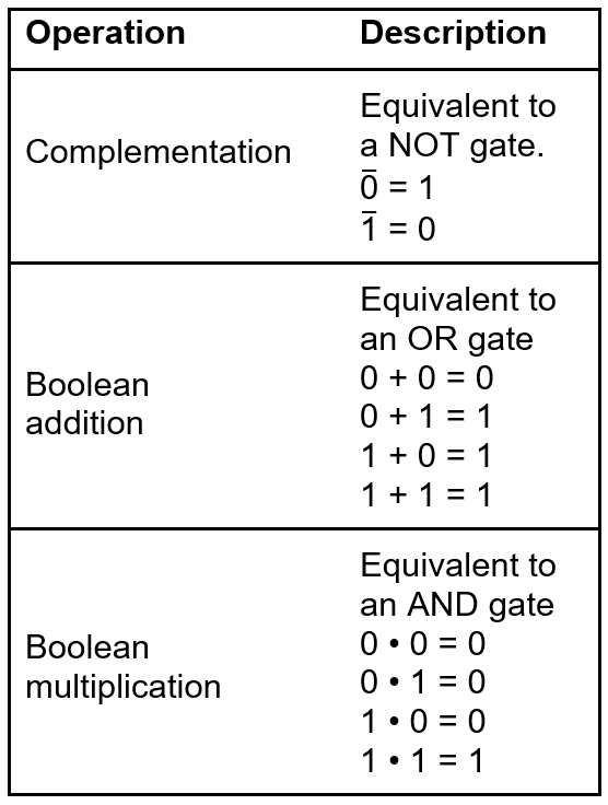
To minimize a standard SOP expression, first perform the process of grouping the 1s. The goal of grouping the 1s is to maximize the size of the groups and minimize the number of groups. For Karnaugh maps of three or four variables, any individual group must consist of 1, 2, 4, 8, or 16 cells. Each cell in a group must be adjacent to one or more cells in the same group (but not all cells in a group need to be adjacent). Each group must contain the largest possible number of 1s. Finally, each 1 on the map must be included in at least one group. Note that a 1 can be included in overlapping groups so long as each of the groups involved also have noncommon 1s. At right, an example of grouping the 1s is displayed.

The next step in minimizing a standard SOP expression is to analyze the groups of 1s. Each group of cells with 1s creates a product term composed of all of the variables in that group which occur in only the complemented or only the uncomplemented form. Any variables which occur in both forms within the group are eliminated. The remaining variables in a given group comprise a term within the minimized SOP expression. All of the terms from the groups are summed to find the full minimized SOP expression.

To use Karnaugh maps with truth tables for standard SOP expressions, place the 1s on the map according to the binary input values and the binary output values described by the truth table (e.g. if the truth table has a value of 101 for the SOP expression AB̅C, put a 1 on the corresponding 101 cell of the Karnaugh map).

Certain binary values are not used in certain applications. For instance, when encoding integers through binary, there are sixteen possible combinations of binary digits but only the integers 0 through 9 need to be represented (ten values). The other six combinations of binary digits are invalid. Since these binary values will never actually occur, their outputs can be treated as either 0 or 1. On Karnaugh maps, these are called “don’t care” terms. “Don’t care” terms are placed on the Karnaugh map as an X and treated as 1 if they help to make a larger group. If a “don’t care” term does not help to make a larger group, it is treated as a 0 output. By helping to make larger groups of 1s, “don’t care” terms can aid in further simplifying SOP expressions and allowing less logic gates to be used.

To map a standard POS expression, place a 0 on the Karnaugh map for each parentheses-enclosed sum term that is part of the expression. Make sure to place the 0s on the cells which match that term of the expression (e.g. (A̅ + B + C̅) goes in the 101 cell of a three-variable Karnaugh map). To map a nonstandard POS expression, it must first be converted to standard POS expression. This conversion is often carried out using a binary-based version of the method outlined earlier.

Karnaugh maps are often used to construct minimized POS expressions (after starting with standard POS expressions). By contrast to standard POS expressions, minimized POS expressions contain the fewest possible terms and the fewest possible variables per term. Minimized POS expressions are usually implementable with fewer logic gates than standard POS expressions.

To minimize a standard POS expression, first perform the process of grouping the 0s. The rules for doing so are identical to the rules for grouping the 1s as outlined in the previous section, except that 0s are used. The next step in minimizing a standard POS expression is to analyze the groups of 0s. This is also carried out in the same way as that described for the SOP version of the process. 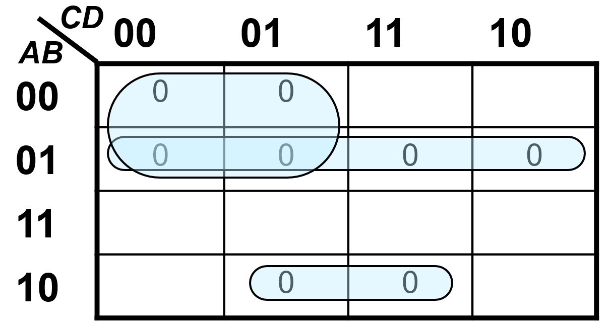After doing this, the remaining variables in a given group comprise a parentheses-enclosed sum term within the minimized POS expression. All of the parentheses-enclosed sum terms from the groups are multiplied to find the full minimized POS expression. “Don’t care” terms are also applied the same way for standard POS expressions as they are for standard SOP expressions.

To use Karnaugh maps with truth tables for standard POS expressions, place the 0s on the map according to the binary input values and the binary output values described by the truth table (e.g. if the truth table has a value of 101 for the POS expression AB̅C, put a 0 on the corresponding 101 cell of the Karnaugh map).

Karnaugh maps can be used to convert between standard SOP and standard POS expressions. This is useful to help compare the minimized versions of the expressions and to see if one of the two can be implemented using fewer logic gates than the other. For going from SOP to POS, all of the cells which do not contain 1s must instead contain 0s. These 0 cells encode the equivalent POS expression. For going from POS to SOP, all of the cells which do not contain 0s must instead contain 1s. These 1 cells encode the equivalent SOP expression.

Basic combinational logic

As described earlier, SOP expressions can be implemented via using AND logic gates as inputs to an OR logic gate output. This is called AND-OR logic. Another important type of logic is using AND logic gates as inputs to an OR logic gate and subsequently inverting the output of the OR gate. This is called AND-OR-Invert logic. To build a XOR gate (referred to as exclusive-OR logic), two AND gates, one OR gate, and two inverters are organized as shown in the figure below. To build a XNOR gate (referred to as exclusive-NOR logic), AND gates, OR gates, and inverters can be organized in multiple ways as shown in the figure below.

Implementing combinational logic from a Boolean expression requires recalling that Boolean multiplication is equivalent to an AND gate, Boolean addition is equivalent to an OR gate, and complementation is equivalent to a NOT gate (inverter). To implement combinational logic from a truth table, first convert the truth table to a Boolean expression via the method described in the truth table section. If a minimized Boolean expression is required, use a Karnaugh map as described in the section on Karnaugh maps.

Universal properties of NAND and NOR gates

The NAND gate is a universal gate because it can be used to make NOT, AND, OR, and NOR functions. The configurations of NAND gates needed to construct these functions are displayed below at left. The NOR gate is a universal gate because it can be used to make NOT, AND, OR, and NAND functions. The configurations of NOR gates needed to construct these functions are displayed below at right.

Combinational logic with NAND and NOR gates

NAND gates can be used to construct AND-OR logic systems (which implement SOP expressions). To do this, connect the output terminals of one or more NAND gates to the input terminals of another NAND gate. Note that the latter NAND gate is acting as a negative-OR gate.

Recall that, when a NAND gate is used to take one or more 0 inputs (i.e. 00, 01, 10 for a device with two inputs), it acts as a “negative-OR” gate. In this case, any of the 0 inputs will give an output of 1, so the operation is similar to OR. Any NAND gate carrying out a negative-OR operation is represented by the alternative symbol at right.

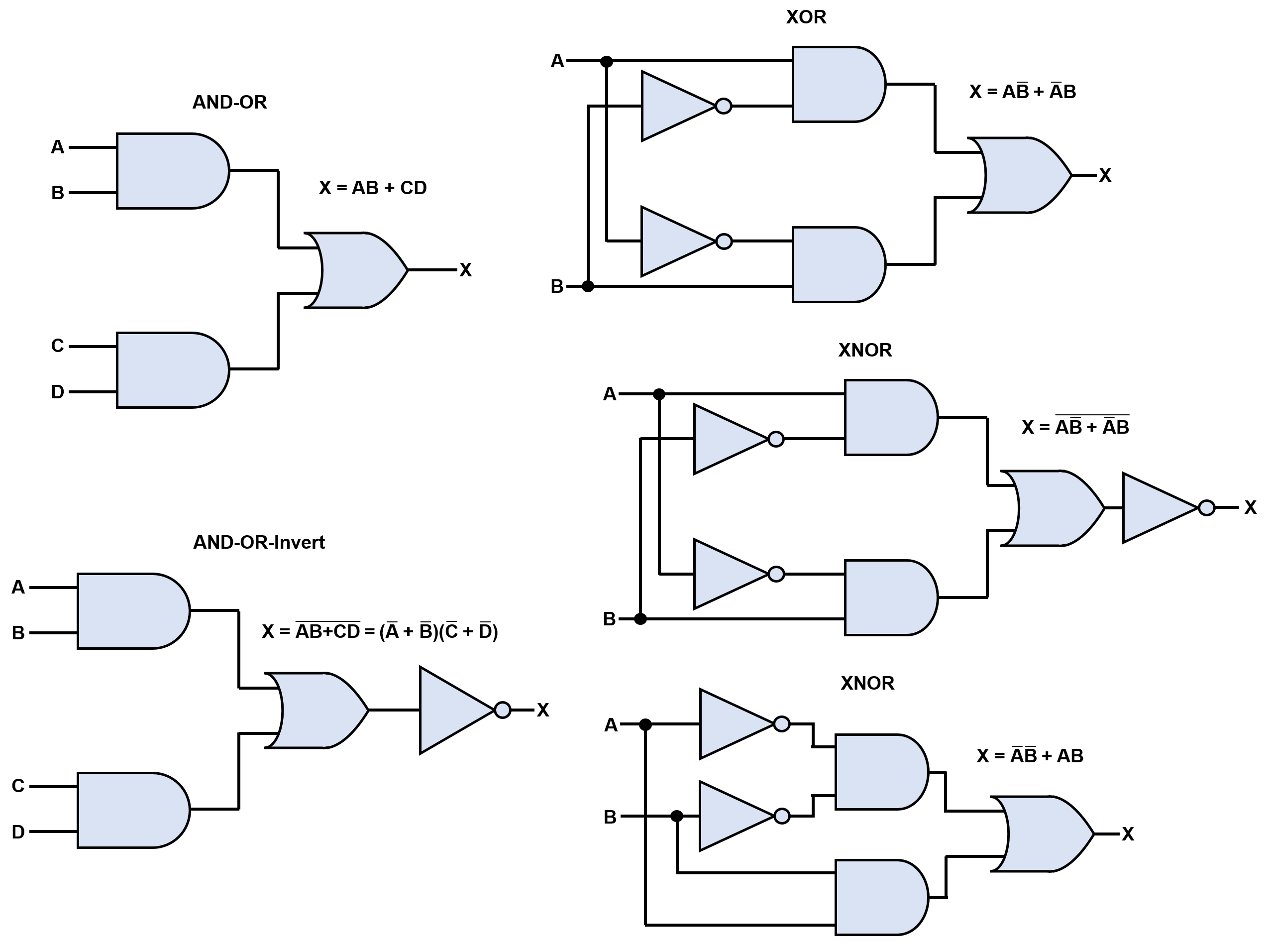
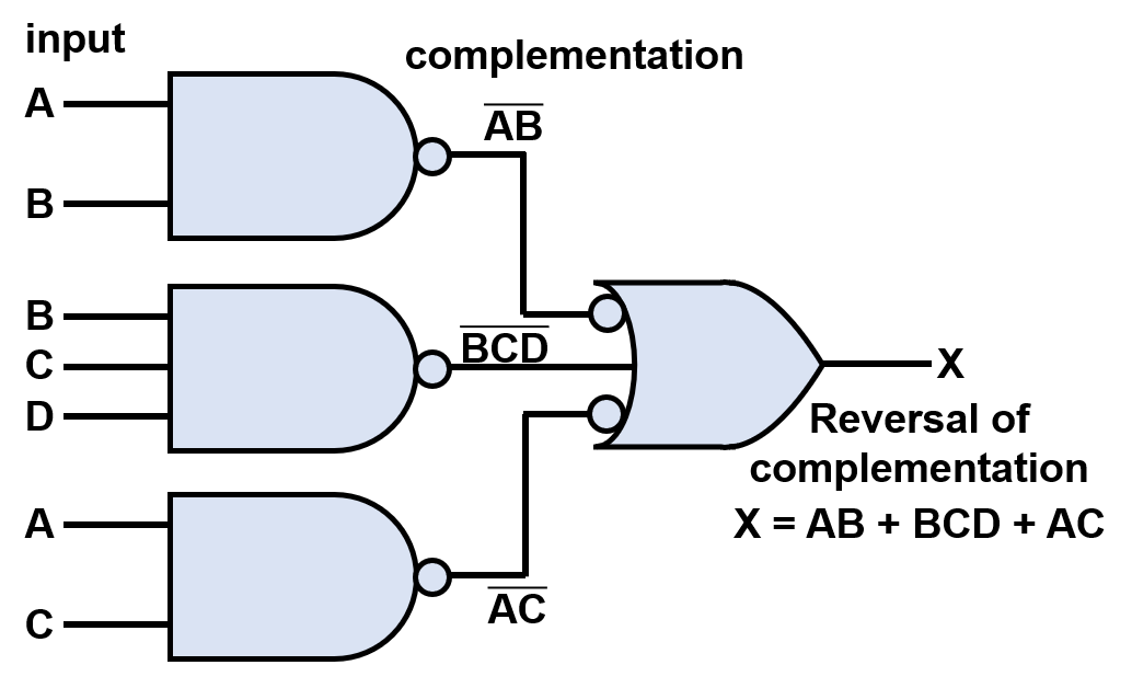When drawing a combinational logic circuit with both NAND gates and negative-OR gates, the symbols should be drawn with NAND gate bubbles facing negative-OR gate bubbles to help make it easier to visualize how the inversion properties of the gates are cancelling each other out (a bubble represents that a gate carries out inversion as at least part of its operation).

NOR gates can be used to construct logic systems which implement POS expressions. To do this, connect the output terminals of one or more NOR gates to the input terminals of another NOR gate. Note that the latter NOR gate is acting as a negative-AND gate.

Recall that, when a NOR gate is used to take all 0 inputs (i.e. 00 for a device with two inputs), it acts as a “negative-AND” gate. In this case, all the 0 inputs together will give an output of 1, so the operation is similar to AND. Any NOR gate carrying out a negative-AND operation is represented by the alternative symbol at right.

When drawing a combinational logic circuit with both NOR gates and negative-AND gates, the symbols should be drawn with NOR gate bubbles facing negative-AND gate bubbles to help make it easier to visualize how the inversion properties of the gates are cancelling each other out. (As mentioned, a bubble represents that a gate carries out inversion as at least part of its operation).

Pulse waveform operation

The voltage or current signals associated with electronic circuits are often represented using trains of pulsed square waves. When a square wave is at its “HIGH” level of voltage or current, it represents a 1. When a square wave is at its “LOW” level of voltage or current, it represents a 0. Although these square waves are ideal forms of messier pulse trains, the binary qualities of digital electronic systems filter out the noise, allowing many analyses to be carried out with ideal square wave pulse trains.

In digital electronics, all waveforms are synchronized to a periodic waveform called the clock which keeps time for the system. All signals within the system are measured against the rate of periodic pulses from the clock. The clock sets the unit of time which denotes a single HIGH or LOW pulse state. This makes it so that the signals can pass through circuit elements (e.g. logic gates) at the appropriate time points and therefore perform appropriate operations.

Timing diagrams compare the signal trains within a digital system. Within each of these units of time, the waveforms for signal trains within the system might take on any combination of HIGH and LOW states.

In the context of logic gates, timing diagrams help to establish what inputs are arriving at which logic gates at what times. To review, the output of an AND gate at a given time is only HIGH if all of its inputs at the given time are HIGH, the output of an OR gate at a given time is only HIGH if at least one of its inputs at the given time are HIGH, the output of a NAND gate at a given time is LOW only when all of its inputs at the given time are HIGH, and the output of a NOR gate at a given time is LOW only when at least one of its inputs at the given time are HIGH.

Binary arithmetic

In digital systems, binary arithmetic serves as an essential mathematical language. It is especially vital for constructing complex combinational logic circuits which perform useful functions. As a starting point, the first fifteen binary numbers are 0, 1, 10, 11, 100, 101, 110, 111, 1000, 1001, 1010, 1011, 1100, 1101, 1110, 1111. These correspond to 1-15 in the base-10 system. Binary uses a base-2 system rather than a base-10 system. As will be explained in the following paragraphs, there are tricks which help to interconvert between binary and base-10 numbers.

The columns of a binary number can be thought of as representing the of base-10 values which sum up to the binary number’s base-10 equivalent where the n^th column from right to left equals 2ⁿ starting with n = 0. To explain this, consider the following example. The binary value of 1011 is equal to eleven in the base-10 system. From right to left, 2⁰•1 + 2¹•1 + 2²•0 + 2³•1 = eleven. This technique can be employed to convert any binary number to a base-10 number. Going the other way, one can convert a base-10 number to a binary number by finding the binary weights w_i that cause the sum of 2ⁿ•w_i to add up to the desired binary value.

To convert a base-10 decimal number to a binary fraction, a similar method is used, but negative binary weights are used for the part of the decimal number which is less than one. For instance, 2^-1 = 0.5 and 2^-2 = 0.25. In addition, a decimal point is inserted into the final binary number and the n within 2^-n grows from left to right. As an example, consider that the base-10 decimal number 0.75 = 2^-1•1 + 2^-2•1, so its binary fractional equivalent is 0.11. Likewise, a binary fraction can be converted to a base-10 decimal number by finding the binary weights w_i that cause the sum of 2ⁿ•w_i + 2^-n•w_i to add up to the desired base-10 decimal number.

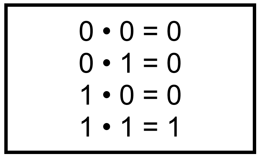
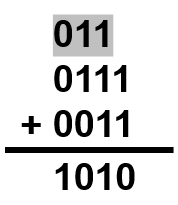Binary addition is summarized in the box below. The top part describes the basic rules for addition of two bits (a bit is a single binary value) and the bottom part describes the rules for the addition of two bits plus a carry bit, which is a value that is carried in the same way as in base-10 addition. The carry bits are highlighted in gray. To illustrate this concept, an example of binary addition with carrying is also shown at right.

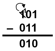Binary subtraction is summarized in the box below. When performing binary subtraction, a borrow is only needed if subtracting a 1 from a 0 digit (e.g. 110 – 1). To borrow, take a 1 from the column to the left, create a 10 in the column undergoing subtraction, and apply the rule 10 – 1 = 1. To illustrate this concept, an example of binary subtraction with borrowing is also shown at right.

Basic binary multiplication rules are summarized in the box below. To multiply two binary numbers, the top number is multiplied by each digit of the bottom number from right to left. The first of these partial products is not shifted left, the second is shifted left by place, the third is shifted left by two places and so on. After shifting, 0 values are put in the empty slots. The partial products are then summed to obtain the result. To illustrate this concept, an example of binary multiplication with shifting is shown at right.

To perform binary division, one must (1) set up long division. The quotient goes on the top, the dividend goes under the quotient, and the divisor goes to the side of the dividend. (2) Place a copy of the divisor below the dividend but align it to the leftmost digits of the dividend. 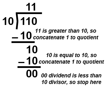(3) If the part of the dividend above the divisor is greater than or equal to the divisor, then subtract the divisor from that part of the dividend, place the result of the subtraction below, and concatenate a 1 to the rightmost end of the quotient. If the dividend above the divisor is less than the divisor, concatenate a 0 to the rightmost end of the quotient. (4) Place another copy of the divisor at the bottom but shift it one column to the right. (5) Repeat steps 3 and 4 until the part of the dividend is less than the divisor. The result is the quotient with the dividend as a remainder. To illustrate this concept, an example of binary division is shown at right.

Half-adders and full-adders

Half-adders take in two input bits and subsequently generate a sum bit and a carry bit, performing the first step in binary addition. Half-adders implement the basic rules of binary addition: 0 + 0 = 0, 0 + 1 = 1, 1 + 0 = 1, and 1 + 1 = 10. Because XOR gates only produce outputs of 1 when the inputs are not equal, a XOR gate is used to generate the sum bit. Because AND gates only produce outputs of 1 when the inputs are both 1, an AND gate is used to generate the carry bit. The truth table for a half-adder is displayed at right. The logic gate diagram for a half-adder is shown below at left and the equivalent logic symbol is shown below at right.

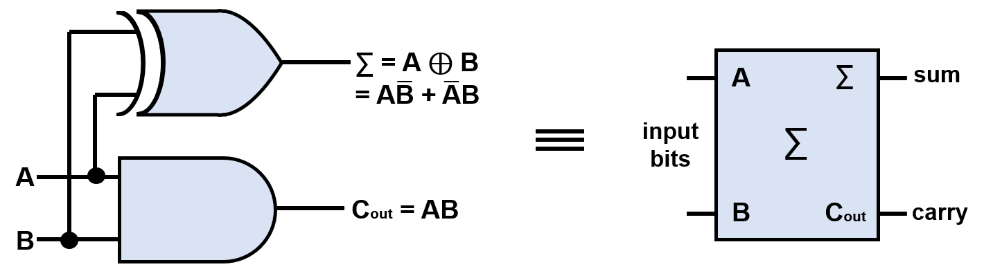
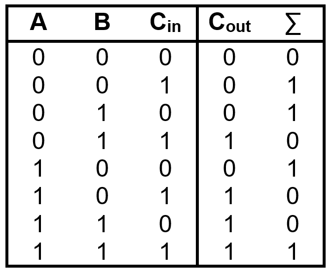Full-adders take in two input bits and an input carry and subsequently generate a sum bit and an output carry before performing the OR operation on them. In other words, full-adders can implement the addition of two 1-bit numbers and an input carry. To see how this corresponds to the rules for binary addition, refer to the box in the section on binary addition. Since the sum of the two input bits is A⊕B, the sum of the two input bits and the input carry is (A⊕B)⊕C_in. (Note that the circled plus indicates the XOR operation). The equation for the output carry is C_out = AB + (A⊕B)C_in. Full-adders are composed of two half-adders and an OR gate. The truth table for a full-adder is displayed at right. The logic gate diagram for a full-adder is shown below at left and the equivalent logic symbol is shown below at right.

Parallel binary adders

Parallel binary adders are composed of two or more full adders and are used to add binary numbers of more than one bit. To add two binary numbers, a full-adder is needed for each bit in the numbers (e.g. for a 2-bit number, two full-adders are necessary). The least significant bit of the output is often grounded to make it zero since there is no carry input to the least significant bit (LSB) position. Note that there is also a most significant bit position (MSB) at the other end of the system. The block diagram for a 2-bit parallel adder alongside the addition operation it performs are shown below.

Extension of these concepts to 4-bit parallel adders and beyond is straightforward. The output carry terminal of each full-adder is linked to the input carry of the next full-adder in the lineup (these links are known as internal carries). In this way, larger binary numbers can undergo the sum operation. As an example, the block diagram for a 4-bit parallel adder and its equivalent logic symbol are shown below.

The truth table for a the 4-bit adder example is shown at right. The subscript n represents the adder bits. C_{n – 1} represents the carry from the previous adder. Carries 1, 2, and 3 are internal carries while carry 4 is an output carry and carry 0 is an input carry.

Ripple carry adders are a category of parallel binary adder which have the output carry of each full-adder connected to the input carry of the next full-adder in the sequence. The sum and the output carry of any stage (a single full-adder is one stage) cannot be produced until the input carry occurs, causing time delays associated with each successive stage. The input carry to the LSB stage must move through all of the stages before a final sum is obtained. Because of this, the cumulative delay is assumed as the number of stages multiplied by the maximum amount of time for the signal to pass through each stage. For an individual ripple carry adder, this cumulative delay is often on the order of tens of nanoseconds.

Look-ahead carry adders are a category of parallel binary adder which eliminate the ripple carry delay and so operate more efficiently than ripple carry adders. To eliminate the ripple carry delay, look-ahead carry adders generate a carry only when both of the input bits are 1s. The input carry then propagates within its full-adder to the output carry. The generated carries are denoted C_g and the propagated carries are denoted C_p. The output carry of a single full-adder can be expressed in Boolean algebraic terms as C_out = C_g + C_pC_in. In parallel binary adders, the C_in of each successive stage equals the C_out of the previous stage. Since each C_g and C_p is expressible in terms of the A and B input bits (to the full-adders), all of the output carries are available almost immediately and it is not necessary to wait for the carries to ripple through all of the stages. The logic gate implementation of a 4-bit look-ahead carry adder is displayed below.

Comparators

Comparators compare two binary numbers and determine relationships between those quantities. The simplest type of comparator decides if two binary numbers are equal. An XNOR gate can act as a comparator to decide if the input bits are equal, giving an output of 1 if the inputs are equal and giving an output of 0 if the inputs are unequal. To expand this to numbers consisting of more bits, the output terminals of multiple XNOR gates are linked to the input terminals of an AND gate. In this way, all of the bits comprising the two numbers must be equal in order for the two numbers themselves to be equal. As an example, a 4-bit comparator and is shown below.

There are also magnitude comparators which can determine whether a binary number is greater than or less than another binary number. To do this, the magnitude comparator must examine if the MSB of number A is greater than, less than, or equal to the MSB of number B. If A_MSB > B_MSB, then A > B, if A_MSB < B_MSB, then A < B, and if A_MSB = B_MSB, then the same process must be performed upon the next most significant bit in the number. The steps are repeated until the relationship between the two numbers is determined. The output which correctly describes the relationship between the two numbers is 1 and the other two outputs are 0. As an example, a logic gate implementation of a 2-bit magnitude comparator and its equivalent logic symbol are shown below.

Decoders

Decoders give an output of 1 when a certain binary number is used as an input and they give an output of 0 for any other binary number input. For example, a decoder might detect the binary number 1001 and output 1 only when the inputs are 1001.

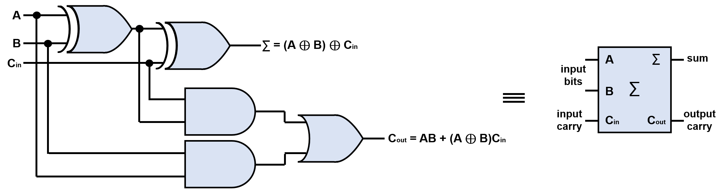
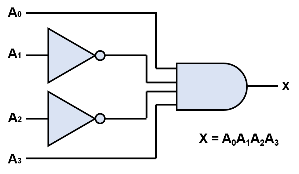To perform their function, decoders must convert all the 0s of the targeted number into 1s via NOT gates and then feed every input to an AND gate. Since the AND gate will only output 1 when all inputs are 1, the targeted number will be detected through the NOT gates converting all 0s in the targeted number to 1s. As an example, the logic gate implementation of a decoder which detects 1001 is shown at right.

One can also construct a decoder using a NAND gate in place of the AND gate. In the NAND gate version, an output of 0 indicates that the specified binary number has been detected.

One common type of decoder configuration is a decoder which takes in n bits and decodes every one of the 2ⁿ possible combinations of those bits. These decoders typically operate by the same principle as described above, though they must send their n inputs to 2ⁿ AND gates or NAND gates (depending on whether the active output needs to be a 1 or a 0). For example, a 4-line-to-16-line decoder receives a 4-bit input and outputs a 1 from a different terminal when it detects each of the 16 distinct combinations of 4 bits. To illustrate this, the truth table of a 4-line-to-16-line decoder which uses AND gates is displayed below.

Because this type of decoder outputs a 1 (or a 0 if NAND gates are used) corresponding to each of the possible 4-bit binary inputs, it can be used to convert 4-bit binary numbers to base-10 numbers. For instance, the binary value 1110 is equivalent to the base-10 value of 14 and 1110 activates the 14^th output terminal. The logic symbol for a 4-line-to-16-line decoder (with 1s as active outputs) is displayed below.

There are other similar decoders that act as standard parts for binary to base-10 conversion. In particular, the BCD-to-decimal converter (“decimal” is another name for base-10 numbers and “BCD” stands for Binary Coded Decimal) or 4-line-10-line decoder uses the same setup as the 4-line-to-16-line decoder, but it only has ten outputs. These ten outputs correspond to the base-10 values of zero through nine. Once again, the active output is 1 if AND gates are used and is 0 if NAND gates are used. Another common decoder is the BCD-to-7-segment decoder, which has a 4-bit input and gives one of seven outputs depending on the input. This decoder also operates on the same principle as the 4-line-to-16-line decoder. However, the BCD-7-segment decoder is used to control the images formed on a seven-segment display device such as a handheld calculator.

Encoders

An encoder first receives an active input on one of its input terminals. The input often represents a digit (such as a base-10 digit), an alphabetic character, or another symbol. Next, the encoder translates this input into a coded output such as a binary value.

One common type of encoder is the decimal-to-BCD encoder. As alluded to in the previous section, BCD code is a way of representing base-10 numbers using 4-bit binary values. The BCD code uses the first ten binary numbers (0000 to 1010) to represent base-10 values of 0 to 9.

The decimal-to-BCD encoder has inputs of 0, 1, 2, 3, 4, 5, 6, 7, 8, and 9 and outputs of A₃, A₂, A₁, and A₀. Decimal-to-BCD encoders use OR gates to convert each input to its appropriate output. The logic of this (assuming 1 as the active value) is as follows. Bit A₃ only outputs a 1 for base-10 digits 8 or 9, bit A₂ only outputs a 1 for base-10 digits 4 or 5 or 6 or 7, bit A₁ only outputs a 1 for base-10 digits 2 or 3 or 6 or 7, and bit A₀ only outputs a 1 for digits 1 or 3 or 5 or 7 or 9. To better understand this, it is helpful to examine the decimal-to-BCD truth table above. The logic gate implementation for a decimal-to-BCD encoder is displayed below alongside its corresponding logic symbol. Note that an input for the base-10 zero digit is not needed since, when all of the binary inputs are 0, the binary outputs are 0000.

Another similar type of encoder is the decimal-to-BCD priority encoder. This type of encoder is configured to include a priority function. As a result, if multiple inputs are given to the decimal-to-BCD priority encoder, the binary output will represent only the largest base-10 value that was used as an input. By comparison, the decimal-to-BCD encoder without the priority function must have only one active input to work properly.

Code converters

It is often necessary in electronic systems to convert between different digital codes. Though there are others, one important type of code converter is the BCD-to-binary converter. This type of code converter can help to illustrate the general idea of code conversion in digital electronics.

From a mathematical standpoint, to perform BCD-to-binary conversion, one must first weight the BCD digits depending on their position within the BCD number. For instance, a decimal value of 27 is represented in BCD as 00100111. In BCD code, the 0010 corresponds to the 2 in the tens place and the 0111 corresponds to the 7 in the ones place. The weights of the tens place are 80, 40, 20, 10 and the weights of the ones place are 8, 4, 2, 1.

In BCD-to-binary circuits, the binary representations of the weights of the BCD bits are added to obtain the corresponding binary number. For the case of 00100111, this is 1•20 + 1•4 + 1•2 + 1•1 = 27 in decimal form and 1•10100 + 1•100 + 1•10 + 1•1 in binary form (the parts that are multiplied by 0 have been excluded here since they equal 0). The BCD-to-binary conversion can be implemented using adder circuits to sum the weighted binary numbers.

Multiplexers

Multiplexers (or data selectors) are devices which take in data from multiple sources and route those data into a single transmission line to send them to a common destination. The way that a multiplexer works is that it receives both data-select lines and data-input lines. Bits sent to the data-select lines control which of the data-input lines is transmitted to the single data-output line.

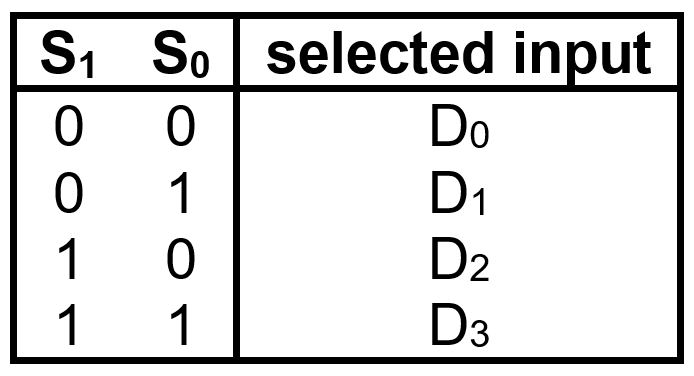As an example, consider a 4-bit multiplexer. The 4-bit multiplexer receives two data-select lines which control four data-input lines. The four possible inputs to the data-select lines (00, 01, 10, and 11) control which of the four data-input lines undergoes transmission to the data-output line. The truth table for this device is displayed at right where S₁ and S₀ are the data-select lines.

To understand how to implement a 4-bit multiplexer using logic gates, it is helpful to see that the Boolean expression below describes the multiplexer’s operation. Y represents the data output. Recall that OR gates implement Boolean addition, AND gates implement Boolean multiplication, and NOT gates implement Boolean complementation. The logic gate implementation and corresponding logic symbol of a 4-bit multiplexer are given along with the Boolean expression.

The principles of 4-bit multiplexers can readily be extended to any n-bit multiplexers. For a given n-bit multiplexer with n data-input lines, log₂(n) data-select lines would be necessary. The logic gate implementation would depend on a Boolean expression analogous to the one above, but with more input variables and more of their corresponding data-select bit combinations.

Demultiplexers

Demultiplexers take information from a single input line and send the information to a given number of output lines. As with multiplexers, demultiplexers also take data-select inputs to determine to which output line the data are sent.

To illustrate how demultiplexers work, consider a 1-line-to-4-line demultiplexer. The logic gate implementation for a 1-line-to-4-line demultiplexer is displayed below. This demultiplexer receives a single data-input line which goes to all of the AND gates. It also receives two data-select lines which control which of the AND gates transmits the data-input line. Since all inputs to an AND gate must be 1 in order for the AND gate to transmit a 1, the data-select lines make it possible to choose which AND gate receives all 1 inputs. Using the data-select lines, only one of the data-output lines will transmit the information at a time.

The principles of demultiplexers in general can readily be found by extending the concept of the above demultiplexer. For a demultiplexer with n data-output lines, log₂(n) data-select lines are needed to control where the data-input line signal is sent.

Modified decoders are also usable as demultiplexers. When a decoder is used as a demultiplexer, its input lines are used as data-select lines since they determine which of the output lines sends an active signal. The modification needed is an enable gate. If the enable gate is not active on both inputs, the decoder cannot transmit any active outputs. By fixing one of the enable gate’s inputs as permanently active, the other input to the enable gate can behave as the data-input line. In this way, the decoder acts as a demultiplexer.

Parity checkers

Parity is a method of error detection. For a given system, any set of bits contains either an even or an odd number of 1s. Depending on the system, the parity bit is attached to a set of bits to make it so that the total number of 1s in the given system is always even or so that the total number of 1s in the given system is always odd. If a system operates with even parity, a parity check is made on each set of bits to make sure that the total number of 1s is even. If a system operates with odd parity, a parity check is made on each set of bits to make sure that the total number of 1s is odd. In the case that these conditions are not met, the system in question reports an error.

To determine if a code has even parity or odd parity, all of the bits in that code are added together. Two bits can be summed using a single XOR gate, four bits can be summed using a pair of XOR gates with their output terminals linked to the input terminals of a third XOR gate, and so on. It is important to note that the sum is a modulo-2 sum. This is a binary sum where a 0 results whenever a carry would otherwise occur (0 + 0 = 0, 0 + 1 = 1, 1 + 0 = 1, 1 + 1 = 0). If a set of bits contains an even number of bits, the XOR gate system will produce a 1. If a set of bits contains an odd number of bits, the XOR gate system will produce a 0. The XOR gate implementations of parity checkers for sets of two, four, and eight bits are given below.

Reference: Floyd, T. (2015). Digital Fundamentals, Global Edition. Pearson Education Limited.

Cover image source: SciTechDaily.com

PDF version: Notes on Optics and Microscopy

Wave optics

The wave equation

Because light exhibits wave-particle duality, wave-based descriptions of light are often appropriate in optical physics, allowing the establishment of an electromagnetic theory of light.

As electric fields can be generated by time-varying magnetic fields and magnetic fields can be generated time-varying electric fields, electromagnetic waves are perpendicular oscillating waves of electric and magnetic fields that propagate through space. For lossless media, the E and B field waves are in phase.

By manipulating Maxwell’s equations of electromagnetism, two relatively concise vector expressions that describe the propagation of electric and magnetic fields in free space are found. Recall that the constants ε₀ and μ₀ are the permittivity and permeability of free space respectively.

Since an electromagnetic wave consists of perpendicular electric and magnetic waves that are in phase, light can be described using the wave equation (which is equivalent to the expressions above). Note that the speed of light c = (ε₀μ₀)^-1/2. Electromagnetic waves represent solutions to the wave equation.

Either the electric or the magnetic field can used to represent the electromagnetic wave since they propagate with the same phase and direction. With the exception of the wave equation above, the electric field E will instead be used to represent both waves. Note that either the electric or magnetic field can be employed to compute amplitudes.

Solutions to the wave equation

Plane waves represent an important class of solutions to the wave equation. The parameter k is the wavevector (which points in the direction of the wave’s propagation) with a magnitude equal to the wavenumber 2π/λ. In a 1-dimensional system, the dot product k•r is replaced by kx. The parameter ω is the angular frequency 2πf and φ is a phase shift.

To simplify calculations, Euler’s formula can be used to convert the equation above into complex exponential form. Only the real part describes the wave as the real part corresponds to the cosine term.

Spherical waves are another useful solution to the wave equation (though they are an approximation and truly spherical waves cannot exist). Because of their geometry, the electric field of a spherical wave is only dependent on distance from the origin. As such, the equation for a spherical wave can be written as seen below with origin r₀.

Gaussian beams are a solution to the wave equation that can be used to model light from lasers or light propagating through lenses. If a Gaussian beam propagates in the z direction, then from the perspective of the xy plane, it shows a Gaussian intensity distribution. For a Gaussian beam, the amplitude decays over the direction of propagation according to some function A(z), R(z) represents the radius of curvature of the wavefront, and w(z) is the radius of the wave on the xy plane at distance z from the emitter. Often these functions can be approximated as constants.

Intensity and energy of electromagnetic waves

The Poynting vector S is oriented in the direction of a wave’s propagation (assuming that the wave’s energy flows in the direction of its propagation).

The magnitude of the Poynting vector represents the power per unit area (W/m²) or intensity crossing a surface with a normal parallel to S. Note that this is an approximation since, according to a quantum mechanical description of electromagnetic waves, the energy should be quantized.

Power per unit area (intensity or irradiance) of plane waves, spherical waves, and Gaussian beams can also be calculated using the equations below. The formula for the Gaussian beam’s power represents the power at a plane perpendicular to the direction of light propagation z.

For electromagnetic waves, instantaneous energy per unit area is difficult to measure, so the average energy per unit area over a period of time Δt is often worked with instead. Since waves are continuous functions, taking their time-average requires an integral.

When using the above integral on the function e^iωt, it is useful to think of finding the real and imaginary parts, cos(ωt) and sin(ωt). Then the time-averages of the cosine and sine functions can be computed using the following equations.

Polarization of light

The waves comprising linearly polarized light are all oriented at the same angle which is defined by the direction of the electric field of the light waves. For linearly polarized plane waves with electric fields oriented along the x or y axes that propagate in the z direction, the following equations describe their electric fields.

The superposition of two linearly polarized plane waves that are orthogonal to each other (and out of phase) is the vector sum of each electric field.

The superposition of two linearly polarized plane waves that are orthogonal to each other (and in phase) is computed via the following equation and has a tilt angle θ determined by the ratio of amplitudes of the original waves. This process can also be performed in reverse with a superposed polarized wave undergoing decomposition into two orthogonal waves.

When two constituent waves possess equal amplitudes and a phase shift of nπ/2, the superposed wave is circularly polarized (as it can be expressed using a sine and a cosine term). Equations for the constituent waves and the superposed wave are given below.

When circularly polarized light propagates, it takes a helical path and so rotates. As such, a full rotation occurs after one wavelength. If a circularly polarized wave rotates clockwise, it is called right-circularly polarized and has a positive sine term. If a circularly polarized wave rotates counterclockwise, it is called left-circularly polarized and has a negative sine term.

If a right-circularly polarized light wave and a left-circularly polarized light wave of equal amplitude are superposed, then they create a linearly polarized light wave with twice the amplitude of the individual waves.

Linearly polarized and circularly polarized light are special cases of elliptically polarized light. For elliptically polarized light, the amplitudes of the superposed waves may differ and the relative phase shift does not need to be nπ/2. As such, the electric field traces an elliptical helix as it propagates along the z direction.

For elliptically polarized light with a positive phase shift φ, it is called right-elliptically polarized if E_0x > E_0y and left-elliptically polarized if E_0x < E_0y.

Most light is unpolarized (or more appropriately, a mixture of randomly polarized waves). To obtain polarized light, polarizing filters are often used.

Superposition of waves with same frequency and direction

Let two waves E₁ and E₂ of the same frequency traveling in the same direction undergo superposition. E₁ and E₂ may or may not possess the same amplitude or phase. The substitution α = –(kx+φ) will be carried out.

If the phases of the waves are different, some special equations are necessary to find the amplitude E₀ and the phase α of the resulting wave.

For the superposition of any number of these waves, the equations above can be extended.

It is often useful to employ complex exponentials when calculating the superposition of waves. For a sum of waves traveling in the same direction which all exhibit the same frequency, the following equation can be used. The summation in parentheses is called the complex amplitude of the resulting wave.

Superposition of waves with different frequencies

In another special case, consider calculation of the superposition of two waves with the same direction and amplitude E₀₁ but different frequencies ω₁ and ω₂. The resulting wave can be expressed using the equation below. Since this wave takes on a beat pattern (see figure), the total disturbance of this wave has an average angular frequency (also called a temporal frequency) of ϖ = 0.5(ω₁ + ω₂) and an average propagation number (also called a spatial frequency) of k̅ = 0.5(k₁ + k₂). The quantity ω_m is called the modulation frequency and the quantity k_m is called the modulation propagation number.

When waves of different frequencies undergo superposition, they create waves which themselves oscillate. The beat pattern is an example of this phenomenon. The smooth curves which outline the extremes of an oscillating signal are called the envelope of that signal.

Often when adding waves of different frequencies, the higher-frequency wave is referred to as the carrier wave and the lower-frequency wave is called the modulating wave. Since the modulating wave determines the envelope of the resulting waveform, this envelope is called the modulation envelope.

Furthermore, when waves of different frequencies undergo superposition, the modulation envelope travels at a different velocity than the constituent waves. The constituent waves travel at their phase velocities, given by v = ϖ/k̅, while the envelope travels at a group velocity. Note that in a nondispersive medium (vacuum), the phase and group velocities are the same since the speed of light is a constant. However, in a dispersive medium (non-vacuum), the phase velocity and group velocities differ. To find the group velocity, the equation below is used. If the frequencies of the two waves undergoing superposition are very similar, then the value of this formula approaches the derivative v_g = dω/dk.

Superposition of waves using Fourier series

Fourier series can be utilized to represent periodic waves. To construct a Fourier series representation of a periodic function of a wave, the following equations are employed. As is consistent, λ is the wavelength and k is the wavenumber 2π/λ. More terms in a Fourier series representation leads to a more accurate approximation of the given wave.

It is often useful to create a Fourier series representation using complex exponentials. To do this, the following equations are used rather than those above.

Interference

Recall that the intensity (or irradiance) of an electromagnetic wave is the power received by a surface per unit area. Due to the high frequencies of many electromagnetic fields, it is often most useful to measure intensity. As such, equations for working with interference and intensity are valuable tools for optics.

When considering the interference of two waves with the same frequency E₁(r,t) and E₂(r,t), the average intensity I_avg of the resulting disturbance over a time period Δt is computed using the following equations. (This treatment assumes that the sources of the waves are separated by a distance much greater than their wavelength). To find I_avg at any given point in space, simply evaluate the equation for I_avg using the coordinates for that point. The angled brackets describe time averages over Δt (recall the integral from a previous section). Here, squaring a vector is equivalent to taking its dot product with itself.

In the case described above, the maximum intensity (total constructive interference) occurs where δ = 2nπ and the minimum intensity (total destructive interference) occurs where δ = (2n+1)π. The light and dark zones that result from constructive and destructive interference are called interference fringes.

For two waves to interfere, they must have the same or very close to the same frequency. In the case of a large frequency difference, a rapidly varying and time-dependent phase difference would occur, causing the interference term (E₀₁•E₀₂)cos(δ) to average to zero. However, when two sources emit white light, some interference takes place. This is because similar wavelengths within the white light will interfere with each other (e.g. blues will interfere with blues). For white light, the interference is not as sharp as in the case of monochromatic light.

Interference patterns will occur when any phase difference between the waves is constant. (Note that two waves with the same frequency and a constant phase difference are coherent waves). In addition, interference patterns are more clearly observable when the interfering waves have very similar amplitudes since this means that the maxima and minima of the interference fringes correspond to total constructive and total destructive interference.

Polarization of light can influence interference. Recall that the polarization state of a wave is defined by the orientation of its electric field. Even if coherent, two waves with orthogonal polarization states cannot interfere. By contrast, coherent waves with parallel polarization states will interfere.

Diffraction

Diffraction occurs when light encounters an obstruction and a multitude of scattered waves result, causing interference patterns to emerge. The vector theory of diffraction is very complicated. But in many applications, one can use approximate scalar treatments of diffraction which are based on Huygens’s principle. When dealing with a viewing position that is close to the obstruction, Fresnel diffraction is used. When dealing with a viewing position that is far from the obstruction, Fraunhofer diffraction is employed.

According to Huygens’s principle, each point on a wavefront can be treated as a source of a secondary spherical wavelet and the envelope of these wavelets describes the new position of the wavefront. One illustrative result of this is that a plane wave passing through an infinitesimal pinhole in a barrier will produce a spherical wave on the other side of the wall. For larger apertures in a barrier, the emerging wave will be the sum of an infinite number of spherical waves originating at each point on the area of the aperture (see figure). It should be noted that the backward propagating part of the secondary wavelet envelope is not physically accurate and is largely ignored in this scalar approximation of diffraction.

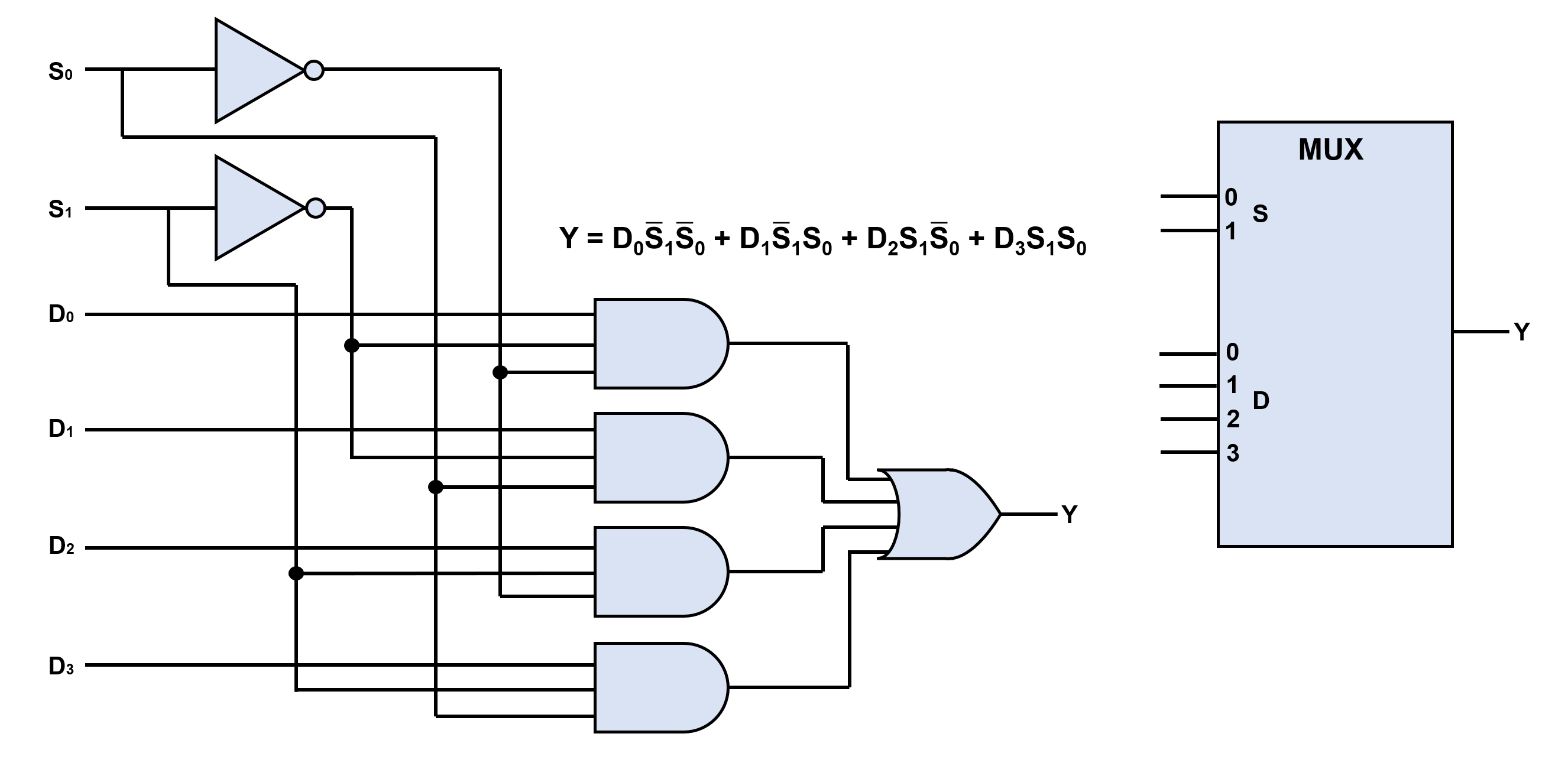
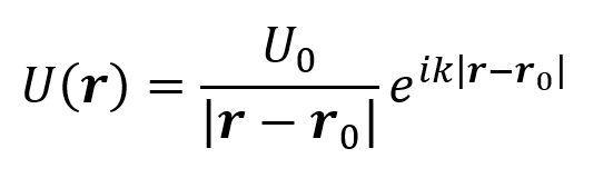
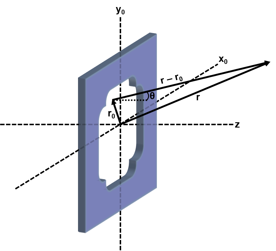For light propagating through an aperture of any shape, the Huygens-Fresnel integral describes the electric field at a point in space r located past the barrier. This integral is an infinite sum of spherical waves that emerge from each infinitesimal point covering the barrier’s aperture. The constant i/λ arises as an approximation of the influence of the angle of the wave arriving at the aperture relative to the aperture’s normal vector. The domain Σ over which integration takes place is the aperture’s area and r₀ represents an infinitesimal surface element of the aperture dx₀dy₀ (with the flat barrier and its aperture described as an xy plane). E_i(x₀,y₀) is the complex amplitude of the incident wave at the point x₀,y₀ on the flat barrier’s xy coordinate system. Here, θ represents the angle of the vector r – r₀ relative to the aperture’s normal vector. A transmission function f(x₀,y₀) can be included inside the integral to describe the effect of a partially translucent surface. For the case of a fully opaque barrier and a fully translucent aperture, f(x₀,y₀) is zero at all barrier points and one at all aperture points. For a system with a partially translucent barrier or aperture, f(x₀,y₀) is a complex quantity with magnitudes falling between zero and one. Recall that the magnitude of a complex quantity a + bi is defined as (a² + b²)^1/2. Though it is an approximation, the Huygens-Fresnel integral is still complicated enough that it is often computed numerically.

The Fraunhofer approximation is employed when the aperture’s size is small relative to the distance to the observation point (such that the light is approximately a plane wave at this observation point). It should be noted that converging lenses can decrease the necessary distance for using the Fraunhofer approximation. Fraunhofer diffraction also assumes that the light source is far enough from the aperture that the incident light can be considered a plane wave. A useful property of the Fraunhofer diffraction integral is that it is mathematically equivalent to a 2D Fourier transform of the aperture’s transmission function f(x₀,y₀). The Fraunhofer diffraction integral equation is given as follows. Here, x₀ and y₀ are points on the plane of the aperture or barrier while r or x, y, and z represent points anywhere in space. 

Ray optics

Refraction and total internal reflection

When light moves between materials with different refractive indices, the refracted ray’s angle changes relative to the incident ray’s angle, a process called refraction. The refractive index n of a material describes the rate of propagation of light within that material relative to vacuum (which has a refractive index of one).

For most media, the refractive index of a given material varies with the wavelength of the light as n(λ). The property of birefringence also occurs in some materials (and is especially common in crystals). Birefringence is when a material’s refractive index varies depending on the angle of light propagation or on the polarization state of the light.

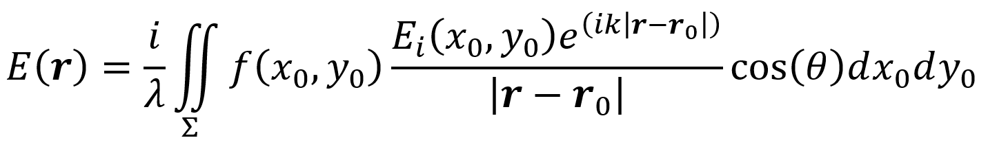
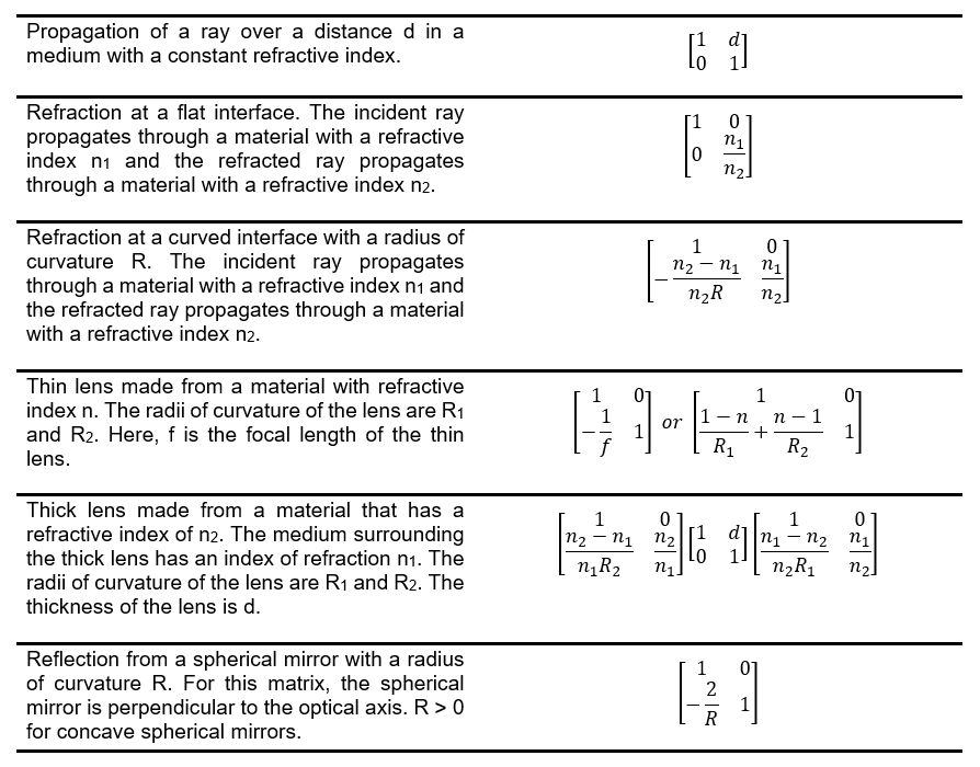
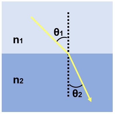Refraction is described by Snell’s law. Here, θ₁ is the incident ray’s angle relative to the normal of the interface, θ₂ is the refracted ray’s angle relative to the normal of the interface, n₁ is the index of refraction of the material in which the incident ray propagates, and n₂ is the index of refraction of the material in which the refracted ray propagates. If n₁ < n₂, the refracted ray bends towards the normal of the interface. If n₁ > n₂, the refracted ray bends away from the normal of the interface. It should be noted that refraction (and reflection) can also be studied in the context of wave optics.

In total internal reflection, a ray of light is reflected from an interface between two media at the same angle as the angle it approached the interface from. Total internal reflection occurs when the incident ray is traveling from a medium with a higher refractive index to a medium with a lower refractive index and approaches from an angle relative to the normal of the interface greater than a value called the critical angle θ_c. The critical angle is computed using the following equation.

Basic ray tracing and lenses

Though ray optics itself represents an approximation and is not as accurate as wave optics, a further simplification called the paraxial approximation is often still useful in practice. For the paraxial approximation, the angles made by all rays with respect the system’s optical axis (e.g. the line perpendicular to a lens) are assumed to be small enough that θ ≈ sin(θ) ≈ tan(θ) and that cos(θ) ≈ 1. This means that Snell’s law simplifies to n₁θ₁ = n₂θ₂.

When working with thin lenses and the paraxial approximation, three rules for ray tracing can be applied. (1) All rays which pass through a focal point on one side of the lens bend as they pass through the lens so that they are parallel to the optical axis when they continue on the other side of the lens. (2) Any ray which passes through the center of a lens continues in the same direction and does not bend. (3) All rays which are parallel to each other (though not necessarily to the optical axis) on one side of a lens will bend as they move through the lens to focus upon a single point on the other side. The location of this point is at the intersection of the optical axis with a ray that both passes through the center of the lens and is part of the group of parallel rays.

The distance d_obj from an object to the thin lens, the distance d_img from the thin lens to where object’s associated image forms, the focal length f of the thin lens, and the magnification M of the thin lens are related using the following equations. The negative value of magnification indicates that the orientation of the image is inverted relative to the object.

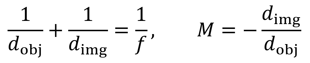
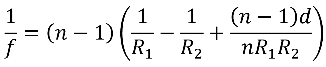
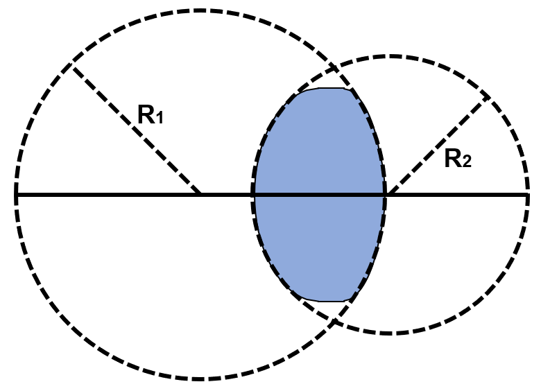The focal length of a thin lens is computed using a simplified form of the lens maker’s equation. R₁ is the radius of curvature for the side of the lens closest to the light source, R₂ is the radius of curvature for the side of the lens furthest from the light source, and n is the refractive index of the material of the lens. Sign conventions for R₁ and R₂ are usually as follows. If the lens is convex, R₁ is positive and R₂ is negative. If the lens is concave, R₁ is negative and R₂ is positive.

For thicker lenses, the full lens maker’s equation is used and takes the following form. Here, d represents the thickness of the lens.

Ray transfer matrix analysis

To aid in the analysis of complicated optical systems, a matrix-based formalism is often employed. Ray transfer matrix analysis requires the paraxial approximation; small enough angles of incident rays relative to the optical axis that θ ≈ sin(θ) ≈ tan(θ) and that cos(θ) ≈ 1). As a result of the paraxial approximation, the equations involved in the propagation of light rays are linear and therefore can be described using matrices. As usual, the propagation direction of rays is conventionally represented as going from left to right.

In ray transfer matrix analysis, a given ray starts out at an angle θ₁ with respect to the optical axis and at a height y₁ relative to the optical axis. After passing through an optical element or a series of optical elements (an optical system), the ray has an angle θ₂ with respect to the optical axis and a height y₂ relative to the optical axis. The ray transfer matrix M (also called the ABCD matrix) helps to compute an output ray from an input ray using an equation of the following form.

The entries of the ray transfer matrix depend upon the components of the given optical system. To describe combinations of several successive optical components, several 2×2 ray transfer matrices are multiplied in the order of the components to give an overall ray transfer matrix. Below is a table of ray transfer matrices for some common optical components.

Fundamentals of Microscopy

Typical organization of a basic light microscope

Modern light microscopes typically employ an objective lens and a tube lens. These are called infinity-corrected microscopes. The objective lens collects light rays and refracts them so that they are parallel to each other. Next, the tube lens focuses these parallel rays onto a detector. The space where the rays are parallel between the objective lens and the tube lens is called infinity space. The magnification of this system is computed by the ratio of the focal lengths of the tube lens and objective lens.

If the microscope allows for direct observation by eye, an extra lens (the ocular lens) refracts the light from the tube lens so that the rays are once again parallel to each other. These parallel rays are subsequently focused onto the retina by the human eye’s lens. The magnification produced by the ocular lens and human eye is the focal length of the ocular lens divided by distance from the eye that the brain perceives the image is located (about 25 cm). Ocular lenses are usually designed to give an additional magnification factor of 10x.

Many microscopes use a detector to carry out imaging rather than (or in addition to) direct observation by eye. Since detectors convert light into an array of pixels using a photodetector array, the size of the individual photodetector devices determines the maximum level of detail that the microscope can acquire. Smaller photodetectors allow for more detail, though this only helps if the microscope’s optics can achieve sufficient resolution to provide this level of detail in the first place. 

Microscopes also require a light source to illuminate the sample. Light sources often pass light through the sample from beneath, though sometimes inverted configurations where the light source is at the top and the objective lens is underneath are used. To focus the light from a source onto a specimen, a condenser lens is employed. In addition, a component called the condenser diaphragm acts as an iris that can adjust the numerical aperture (a concept described in the next section) of the condenser lens by limiting the size of the light cone.

Resolution in light microscopy

The maximum angle at which rays from the specimen can be collected by the objective lens is called the angular aperture. Using the angular aperture, the numerical aperture NA of the objective lens is computed. Numerical aperture is important for calculating the resolution of a light microscope. Here, n is the refractive index of the medium between the lens and the specimen and α is half of the angular aperture.

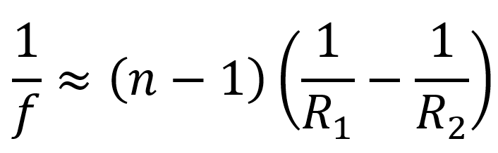
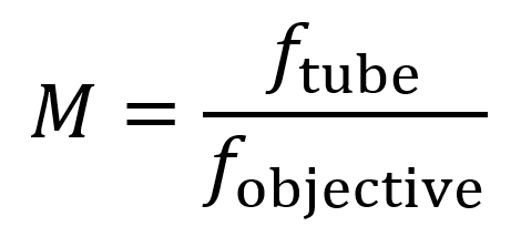
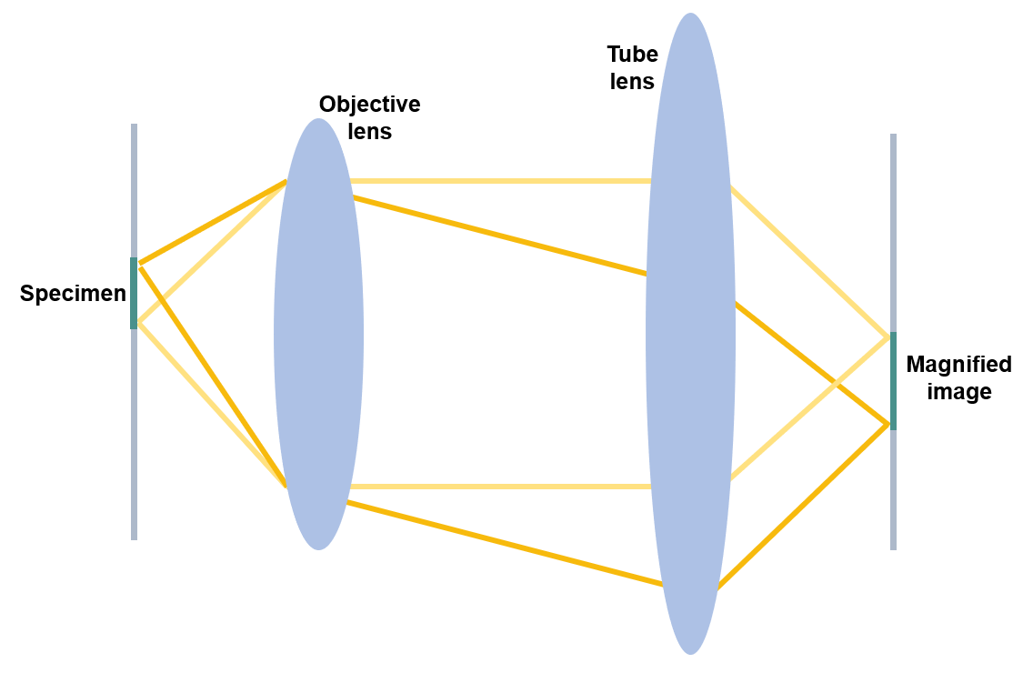
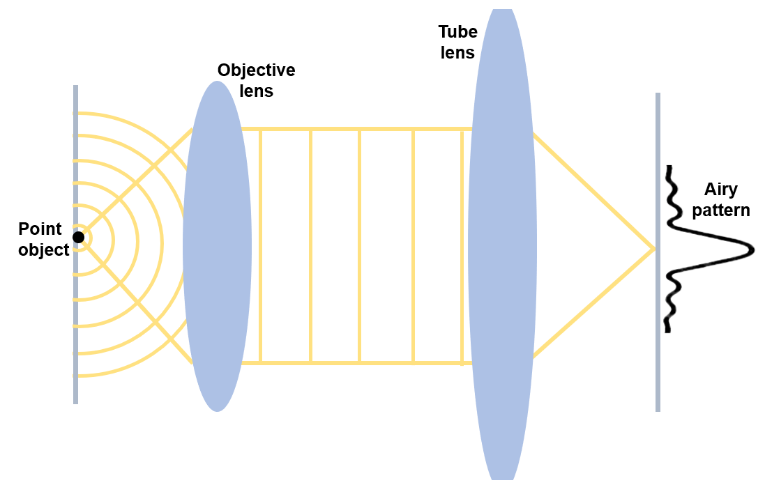The resolution of light microscopy is diffraction limited (except in super-resolution microscopy), meaning that diffractive effects result in a maximum achievable resolution which depends on wavelength and numerical aperture. To understand this, consider diffraction from a point object. (Assume small angles with respect to the optical axis and neglect vector analysis). According to Huygens’s principle, the point object diffracts incoming light into a spherical wave. Part of this spherical wave is converted into a plane wave by the objective lens. Next, the tube lens focuses this light. At the focus on the image plane, the waves constructively interfere since they exhibit the same optical pathlength. But around this point, the optical pathlengths are different and a series of concentric circles of destructive and constructive interference occur. This phenomenon is called the Airy pattern.

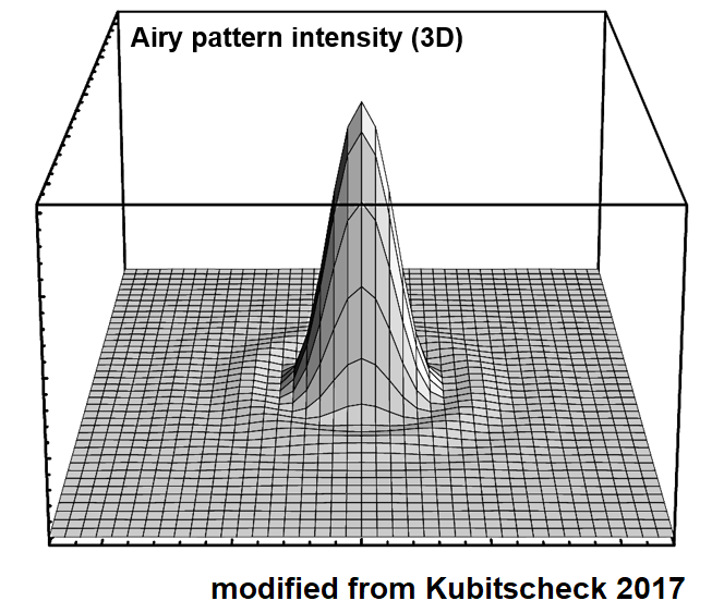The intensity of light from the Airy pattern is a type of point spread function (PSF). Any microscope image is made up of a tapestry of PSFs. It should be noted that the Airy pattern represents an ideal PSF for a perfect optical system and that many other kinds of PSF exist. By using the Fraunhofer diffraction integral and integrating over a circular aperture (the objective lens) with radius a, the Airy pattern’s field is calculated as a function of the angle θ between the optical axis and the line from the center of the aperture to the observation point (see the figure in the diffraction section for a visual depiction of θ). The function for the Airy pattern’s intensity can be computed by squaring the equation of the field. Here, J₁ represents a type of function called a Bessel function of the first kind of order one. I₀ is the maximum intensity at the Airy pattern’s center.

The reason the Fraunhofer integral can be used is that the refraction of the spherical wave into a plane wave makes the component waves parallel such that the image plane is effectively at the far field. Also note that the radial symmetry of the Airy pattern allows for I(θ) to describe the pattern in 3D despite only depending on a single variable.

Since microscope images are made up of a tapestry of PSFs as mentioned above, PSFs are useful in helping to describe resolution. As a type of PSF, the Airy pattern is often used to help calculate resolution. The circular region of the Airy pattern with a radius defined by the distance between the intensity distribution’s central maximum and its first zero is called the Airy disk.

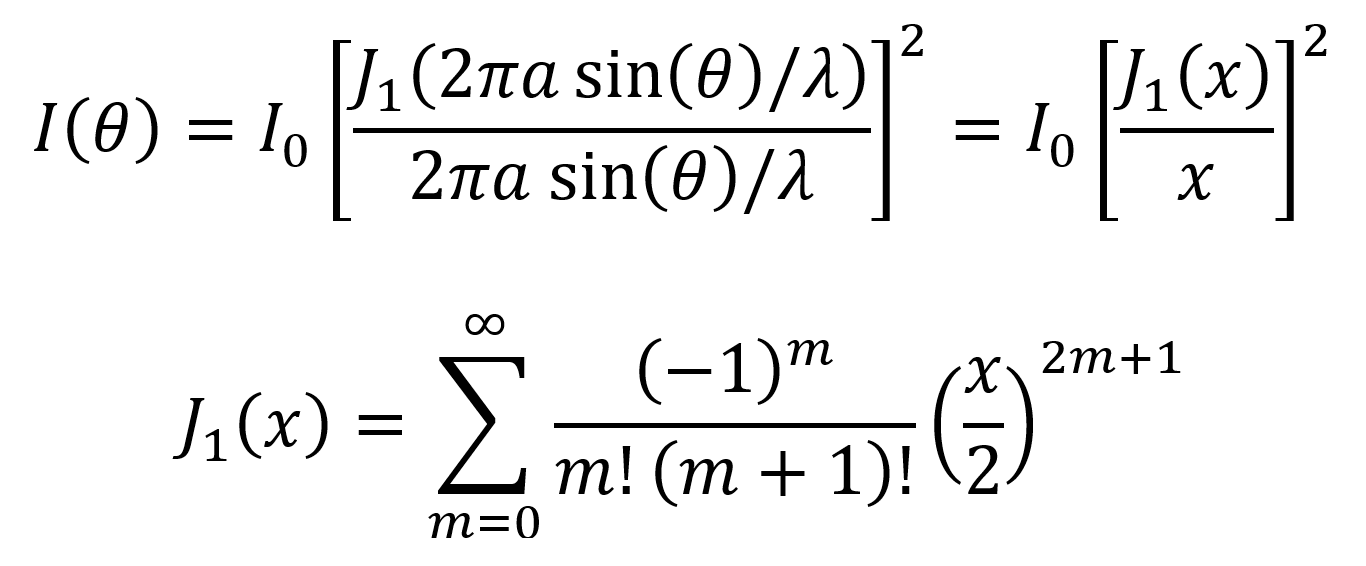
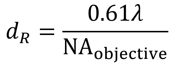
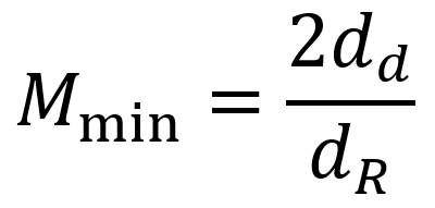
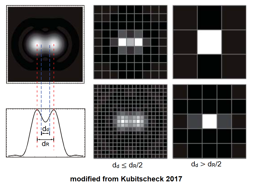
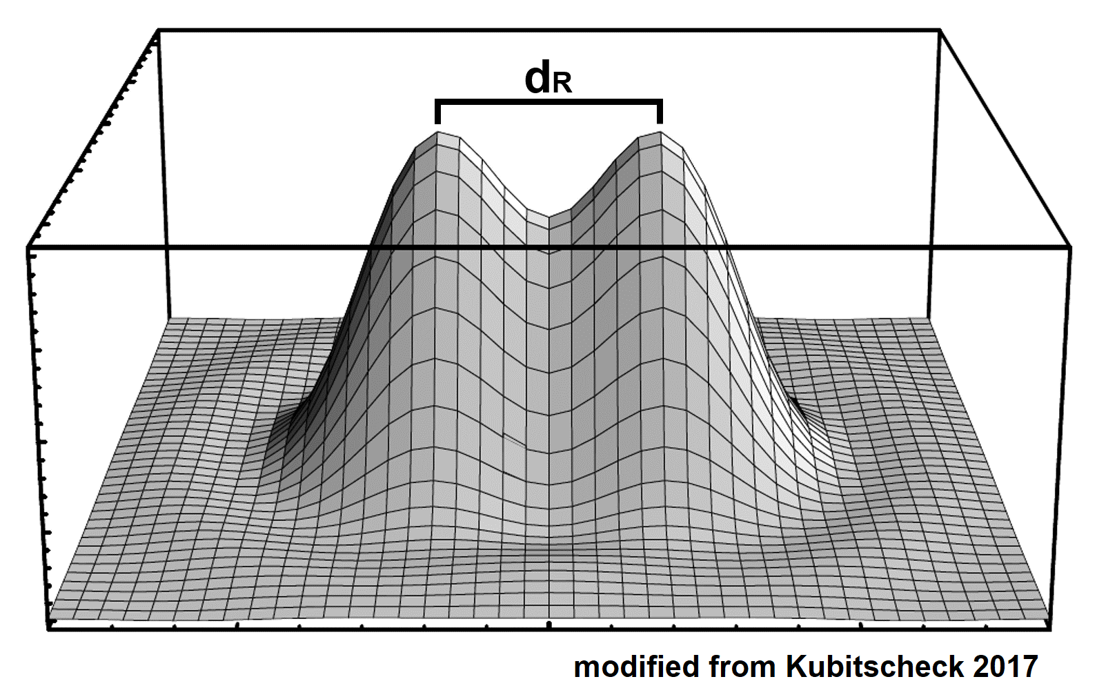If two point objects are farther from each other than the radius of the Airy disk d_R (which depends on wavelength and numerical aperture, they are perceivable as separate objects. This principle is used as a measure of lateral resolution (x and y directions) and is called the Rayleigh criterion. Note that there are also other measures of lateral resolution such as the Sparrow limit.

When the light source illuminating the object uses coherent light (where waves exhibit the same frequency and a constant phase difference), the Rayleigh criterion is given by the following equation. Laser-based light sources and situations in which the condenser aperture is closed to produce a pointlike light source are the most common type of coherent light sources used in microscopy. In the case of the narrow condenser aperture, the numerical aperture of the condenser is sometimes approximated as zero.

In the cases where incoherent light is involved, the situation is different since the light between two adjacent points does not interfere. This happens when the sample itself emits light (as in fluorescence microscopy) or when the numerical aperture of the condenser lens is greater than or equal to the numerical aperture of the objective lens, the Rayleigh criterion is given by the following equation.

Measuring axial resolution in a manner that is consistent with the Rayleigh criterion requires using the intensity distribution of light along the optical axis (z direction). This axial interference pattern is typically hourglass shaped. However, it still exhibits a central maximum as well as regions of minimum intensity along the z axis. The distance between the central maximum and the first minimum is used as an approximate measure of axial resolution. This distance can be computed using the following equation. Here, n is the refractive index of the immersion medium between the specimen and the objective lens.

As mentioned earlier, the size of the individual photodetector elements in a microscope’s detector array determines the maximum possible level of image detail. To collect all of the available information from an image, the size d_d of each photodetector element must be at most half the resolution or radius d_R of the Airy disk in the image plane (that is, d_d ≤ d_R/2). Because the microscope’s magnification makes the specimen appear larger, it also multiplies the apparent radius of each Airy disk. This means that a higher magnification factor will cause each Airy disk to cover a larger number of photodetector elements (and pixels). As such, the minimum magnification factor necessary to make it so that d_d ≤ d_R/2 is given by the following equation.

Lens aberrations

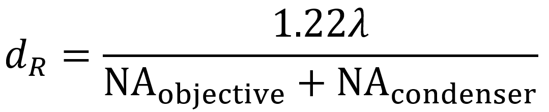
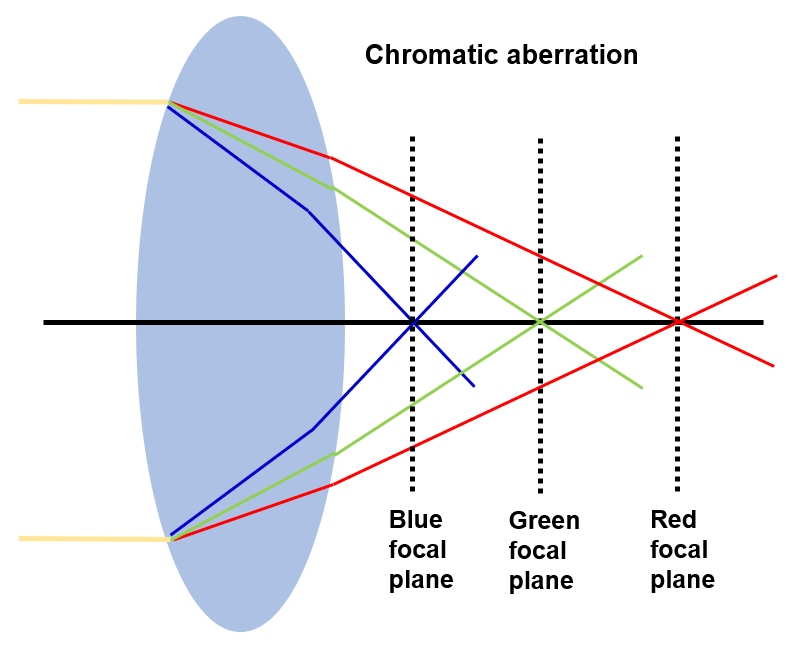Because the refractive index of a lens is wavelength dependent, different colors of light passing through the lens refract at different angles and create distinct focal planes. This causes lens aberrations that are known as chromatic aberrations.

Most lenses have spherical curvature since lenses with other types of curves are much more difficult to manufacture. Note that this does not necessarily mean these lenses are entirely spherical, just that the curved surfaces on the lenses could act as parts of a sphere. Unfortunately, light refracts at different angles towards the edges of these kinds of lenses. This is a result of the angle of incidence for parallel rays changing with the increasing curvature near the edges. With different angles of refraction, distinct focal planes occur, producing lens aberrations called spherical aberrations.

Any curved lens does not produce a flat focal plane, but rather a bowl-shaped focal region. Since microscopy often involves imaging samples with mostly flat geometry (e.g. samples on glass slides), this bowl-shaped focal region leads to a type of aberration known as a field curvature aberration.

When there is a disparity between the focal distances of rays passing through the vertical and axis of a lens and the horizontal axis of the lens, it leads to poorer image quality, focuses point objects as streaks, and is called astigmatism. This aberration sometimes comes from differences in vertical curvature and horizontal curvature of a lens due to imperfections in manufacturing. But even in a lens with perfect symmetry, when the object under observation is located away from the optical axis, a form of astigmatism called oblique astigmatism can occur (which has the same effect of creating distinct focal planes for the horizontal and vertical axes of the lens). The further the object is from the optical axis, the more severe the oblique astigmatism.

Slightly tilted lenses can result in an aberration known as coma. With coma, a cometlike blur oriented either away from the optical axis (positive coma) or towards the optical axis (negative coma) occurs.

Types of objective lenses

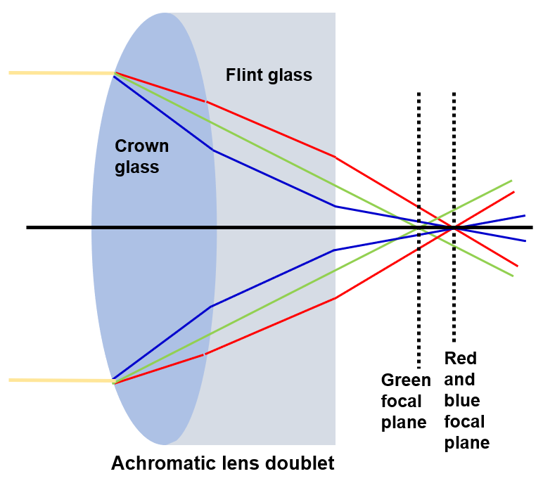To correct for chromatic aberrations which arise between two wavelengths of light (usually blue and red), compound lenses made from materials with different dispersion properties are used. These lenses are called achromatic lenses (or achromats). Dispersion refers to the wavelength dependence of refractive index. Achromatic objective lenses typically employ convex lenses made from crown glass fused to concave lenses made from flint glass, though the entire objective often involves more than just this lens doublet. The differences in dispersion (and therefore refraction) resulting from the crown glass and flint glass cancel each other out, correcting for chromatic aberrations in two wavelengths and creating a single focal plane for both of these wavelengths of light. In addition, achromatic objectives correct for spherical aberrations in a single wavelength which lies between two chromatically corrected wavelengths.

When correcting for chromatic aberrations between blue, red, and green wavelengths, a fluorite lens is often employed. Fluorite objectives are typically similar to achromatic objectives (in that they include fused convex and concave lenses), but they use convex lenses made from fluorite glass rather than flint glass. Though usually more expensive than achromats, the dispersion properties of the convex fluorite glass is better able to complement the material of the concave lens, leading to a single focal plane for red, blue, and green light.

Apochromatic objectives are very expensive and combine many individual lenses so as to correct for chromatic aberrations in four or even five wavelengths such as red, green, blue, near-UV, and near-infrared. They are also typically corrected for spherical aberration in green and blue wavelengths. Some apochromatic objectives are constructed to exhibit minimal field curvature and are called plan-apochromats.

There are also special objective lens designs for various applications. Some examples include long working distance objective lenses, immersion objectives (immersion of an objective in liquid often creates a closer refractive index match to the lens material and improves image quality), and UV-transparent objectives to support uses that involve ultraviolet light.

Mirrors

Many optical microscopy setups are complicated and require mirrors to direct light to the necessary locations. Mirrors are also used for many other purposes in microscopy (e.g. curved mirrors can spread light out, etc.) Reflectance, the ratio of reflected light to incident light, is used to quantitatively evaluate the performance of mirrors. The angle at which a ray of light undergoes reflection is equal to the incident ray’s angle relative to the normal of the mirror’s surface. The reflected ray travels away from the mirror on the opposite side of the normal.

Metallic mirrors are made by coating a substrate with a thin layer of metal. The electrons in metallic substances are not bound to any one atom, so they are free to move through a metal’s volume. As such, metals electromagnetic fields induce oscillations in these free electrons. The oscillations cause reemission of the wave with a 180° phase shift relative to the incident wave, leading to destructive interference along the direction of the incident wave’s propagation. Due to the destructive interference, the reflected wave does not transmit into the metal, only out from the surface.

Many metallic mirrors can achieve 90-95% reflectance depending on what material they are made from. However, there are tradeoffs since a metallic mirror’s reflectance can rapidly decrease outside of a certain wavelength range. For instance, silver shows around 95% reflectance across visible and infrared spectra but drastically lower reflectivity in the ultraviolet region. The reflectance R of a metallic mirror can be computed (as a proportion) using the equation below where n is the metallic coating’s refractive index and ε is the metallic coating’s molar extinction coefficient. The molar extinction coefficient is a measure of how strongly a material attenuates light at a given wavelength.

It should also be noted that the molar extinction coefficient can be found experimentally by using absorption spectroscopy and applying the Beer-Lambert law. The Beer-Lambert law is given below where L is the optical pathlength (the distance that light travels from one side of the sample to the other side), c is the molar concentration of the substance, and A is the measured absorbance.

Dielectric mirrors take advantage of the fact that nonmetallic materials exhibit some reflectivity. To make a dielectric mirror, alternating layers of materials with low and high refractive indices are deposited on top of a substrate. Partial reflection occurs at the interfaces between the layers. Because the many layers each contribute some reflection, the total reflectance of a dielectric mirror can exceed 99%. Dielectric mirrors are often used with laser sources.

For a dielectric mirror, the thicknesses and refractive indices of its layers allow tuning of the mirror’s properties. Some designs can reflect only a narrow range of wavelengths while others can reflect a broad range of wavelengths.

Dielectric mirrors that reflect a specific wavelength (or range of wavelengths) are often designed such that the thickness times the refractive index of each layer equals one quarter of the target wavelength. Layers with alternating low and high refractive indices are still used, so the thicknesses are varied accordingly. As a result, constructive interference occurs among the partially reflected waves at the interfaces between each layer, adding up to achieve a high level of reflectance. It should be noted that dielectric mirrors are sensitive to the angle of incidence and therefore require correct positioning to function properly.

One useful type of dielectric mirror is a dichroic mirror. These dichroic mirrors reflect a designated range of wavelengths and transmit colors (through the mirror) which fall outside of this range. To do this, the thicknesses and refractive indices of the layers are adjusted so as to cause constructive interference which reinforces wavelengths that fall within the desired range.

Though mirrors are often flat, curved mirrors are also common in microscopy. They are used to bend the paths taken by light, for focusing light, to magnify or reduce images, and other applications. Curved mirrors come in a variety of shapes (e.g. with spherical, parabolic, or hyperbolic curvature) and can have concave or convex geometry.

Curved mirrors can behave similarly to lenses, reflecting light rays to converge at a certain focal distance f. As a result, the mirror equations are identical to the thin lens equations (see below). Recall that this assumes the paraxial approximation. When the object or image is in front of the mirror the value of d_obj or d_img is positive. When the object or image is behind the mirror the value of d_obj or d_img is negative. Using these sign conventions along with ray tracing methods, the mirror equation can be applied to both concave and convex mirrors.

There are several useful concepts to note with regards to the properties of particular types of curved mirrors. Spherical mirrors have a focal length equal to half the radius of curvature. Concave cylindrical mirrors reflect light into a linear focal plane. Concave paraboloidal mirrors focus plane waves into a point source and can also convert a point source into a plane wave.

Sources

For fluorescence microscopes, there are usually two light sources. One is a standard halogen lamp that allows a user to view the specimen using light transmission rather than fluorescence. The other is a more specialized and much brighter light source used for exciting fluorophores, sometimes a mercury arc lamp, a xenon arc lamp, a metal halide lamp, or a laser source.

Mercury arc lamps, xenon arc lamps, and metal halide lamps emit light across a wide range of spectra, though they each exhibit some specific differences in their emission ranges and peaks as seen in the following figure. It should be noted that metal halide lamps have a longer lifetime than mercury arc lamps and xenon arc lamps. Unfortunately, these types of light source do not emit light with constant intensity in space and time. Photons undergo emission in bunches rather than in a uniform series, fluctuations in the lamp’s temperature and in the lamp’s electric current can cause emission inhomogeneities, and external electric fields can interfere with the uniformity of emission. These issues can sometimes cause problems in quantitative microscopy.

Lasers provide more stable illumination. Lasers that emit single wavelengths as well as lasers that emit a broad spectrum of wavelengths are available. Lasers use a process called stimulated emission to produce light. Stimulated emission involves external electromagnetic radiation causing excited electrons to transition to their ground states more frequently than they would otherwise, causing emission of photons. An important property of stimulated emission is that the emitted photons exhibit the same direction, frequency, phase, and polarization as the incident electromagnetic radiation.

References

Boudoux, C. (2017). Fundamentals of Biomedical Optics. Blurb, Incorporated.

Degiorgio, V., & Cristiani, I. (2015). Photonics: A Short Course. Springer International Publishing.

Guenther, R. D. (2019). Modern Optics Simplified. Oxford University Press.

Hecht, E. (2017). Optics. Pearson Education, Incorporated.

Kubitscheck, U. (2017). Fluorescence Microscopy: From Principles to Biological Applications. Wiley.

Murphy, D. B., & Davidson, M. W. (2012). Fundamentals of Light Microscopy and Electronic Imaging. Wiley.

Cover image source: Nature

PDF version: Primer on the Biology of the Cerebral Cortex

Cortex cytoarchitecture

On the axial dimension, the cerebral cortex is partitioned into six layers of cells. Layer 1 of the cerebral cortex is the most superficial and layer 6 is the deepest relative to the surface of the brain. Layers 2 and 3 are often categorized together as layer 2/3. Laterally, the cerebral cortex is tiled by distinct regions called cortical columns which act as repeating units of similar function.

Layer 1 and layer 2/3 are called the supragranular layers and mostly perform intracortical computations. Layer 4 is called the granular layer and functions primarily to receive thalamic input. Layers 5 and 6 are called the infragranular layers and mainly send outputs to other parts of the brain.

Though the majority of cortical cells are excitatory pyramidal neurons, there are also many inhibitory interneurons which are crucial to cortical function. There are many morphologically distinct classes of inhibitory interneurons. Pyramidal cells also exhibit structural diversity, though their morphological differences are less often discussed in an explicit fashion.

Canonical cortical microcircuit 

The canonical cortical microcircuit is a model for some of the most frequently occurring patterns of cortical connectivity and function. Some neuroscientists hypothesize that most cortical circuits are variations of a canonical microcircuit. Though different authors have suggested somewhat different versions of the canonical cortical microcircuit model, there are some common patterns as follows.

According to the canonical cortical microcircuit model, strong thalamic inputs first arrive at layer 4 and stimulate both the layer’s inhibitory interneurons and its excitatory pyramidal neurons. Next, these layer 4 neurons transmit information to layer 2/3 pyramidal cells which in turn send excitatory projections to layers 5 and 6 (as well as to layer 1). Layers 5 and 6 send both excitatory and inhibitory signals to other parts of the brain (e.g. back to the thalamus, to the brainstem, etc.) Layers 5 and 6 also send both excitatory and inhibitory feedback to layer 4.

Cortical hierarchy and extrinsic connections

Links among neurons within a cortical column are referred to as intrinsic connections while links between neurons in different cortical columns are called extrinsic connections. Though the majority of cortical connections are intrinsic, the extrinsic connections often stimulate (via activation and inhibition) their targets more strongly.

There are three types of extrinsic connections; feedforward, feedback, and lateral connections. Feedforward connections are from supragranular pyramidal cells to layer 4, feedback connections are from infragranular pyramidal cells to any layer except layer 4 (usually the supragranular layers), and lateral connections are between cells in the same layer. By using this laminar system, a cortical hierarchy emerges with lower cortical areas such as V1 sending information to higher cortical areas such as the dorsal and ventral visual streams via feedforward connections.

Feedback connections are usually inhibitory and can be either modulatory or driving. Though only excitatory lateral connections are shown in the figure above, lateral connections vary in whether they are excitatory, inhibitory, modulatory, or driving. Modulatory connections produce weak metabotropic and ionotropic responses while driving connections produce strong ionotropic responses.

Extrinsic connections are mostly from excitatory glutamatergic neurons, yet feedback connections are usually inhibitory. As such, it is thought that feedback connections typically involve excitatory neurons stimulating layer 1 cells which subsequently send inhibitory projections to layer 2/3 pyramidal cells.

Feedforward connections are excitatory and driving. Feedforward connections might operate as either corticocortical links or as transthalamic links. Transthalamic refers to when a cortical projection goes to the thalamus and then the postsynaptic thalamic neuron sends an axon back to some other part of the cortex.

Reference: Bastos, A. M., Usrey, W. M., Adams, R. A., Mangun, G. R., Fries, P., & Friston, K. J. (2012). Canonical Microcircuits for Predictive Coding. Neuron, 76(4), 695–711. https://doi.org/https://doi.org/10.1016/j.neuron.2012.10.038

Cover image: modified from Innovations Report article on Motta et al.’s paper